Calculus I Notes

Math 141 - Spring 2024

Week 1 Notes

Wed, Jan 17

Today we reviewed functions and function notation. We talked about how $f(x)$ looks like $f$ multiplied by $x$, but it really means something completely different! We also talked about the following important functions (and their graphs) that you should have memorized:

1. Linear functions $f(x) = mx+b$.

2. The square function $f(x) = x^2$.

3. The positive square-root function $f(x) = \sqrt{x} = x^{1/2}$.

4. The reciprocal function $f(x) = \dfrac{1}{x}$.

5. The 1-dimensional distance function $f(x) = |x-a|$.

We reviewed the definitions of domain, range, and function composition. We did the following examples in class.

1. Let $f(x) = \dfrac{4}{x+2}$ and $g(x) = \dfrac{1}{x}$. Find the domain of $f(g(x))$. (https://youtu.be/PNzHrPebKOw)

2. Two poles are connected by a wire that also connects to the ground between the poles. Find a formula for the length of the wire as a function of $x$ and determine the domain.

We didn’t have time for this exercise, but it is also a good example of how to construct a function.

3. A rectangular piece of cardboard is 10 inches by 8 inches. If we cut squares of length $x$ out of the four corners, then we can fold the sides up to make a box. Find a formula for the volume of the box as a function of $x$ and determine the domain. (https://youtu.be/UvTYc5Wqu8w)

Thu, Jan 18

Today we started with the wire between two poles example from yesterday. Then we focused on linear functions. We reviewed slope-intercept form and did the following examples in class.

1. Find the formula to convert Celsius temperatures to Fahrenheit.

2. Find a formula for the line through $(4,9)$ and $(6,1)$. (https://youtu.be/LtpXvUCrgrM)

As of 2023-24, the US Income Tax brackets for individuals earning up to $95,375 are:

3. Express income tax owed as a function of income for individuals earning up to $44,725.

Here is another good example that we didn’t do in class:

4. Find the slope and intercepts of $3x+5y = 15$. (https://youtu.be/SOwh-Wk7Cq0)

Fri, Jan 19

Today we talked about polynomial functions and equations. We briefly reviewed how to factor polynomials and we solved the following problems.

1. Suppose $f(x) = x^2$ and $g(x) = 5x-6$. Find the $x$-values where these two functions intersect.

2. Solve $x + \dfrac{8}{x} = 6$. (https://youtu.be/1fR_9ke5-n8?t=112)

3. Solve $\dfrac{x^2}{4} = \dfrac{2x}{x-6}$.

In the last example, you should get to $x(x^2 - 6x - 8) = 0$. Unfortunately there aren’t integer factors of $-8$ that add up to $-6$. So you need to use the quadratic formula $$x = \frac{-b \pm \sqrt{b^2 - 4ac}}{2a}$$ to find all of the solutions. You do not need to memorize the quadratic formula (it will be on the formula sheet on exams and you can look it up when you are doing your homework if needed).

Week 2 Notes

Mon, Jan 22

Today we did a review of some basic trigonometry. We talked about the things you should memorize which include:

• $\pi$ radians is 180 degrees.
• The definitions of sine, cosine, and tangent (SOH-CAH-TOA).
  
• The graphs of $\sin(x)$ and $\cos(x)$.

We did the following exercises.

1. Convert $\tfrac{-\pi}{3}$ radians to degrees. (https://youtu.be/z0-1gBy1ykE)

2. Convert $150^\circ$ to radians. (https://youtu.be/O3jvUZ8wvZs)

3. Find the values of $\cos \theta, \sin \theta, \tan \theta, \sec \theta, \csc \theta,$ and $\cot \theta$ for the angle $\theta$ shown below.

3. Find $\sin(\tfrac{4\pi}{3})$. Hint: use the formula sheet.

4. Find $\cot(-\tfrac{2\pi}{3})$ (https://youtu.be/KaS3P1a7GE8)

5. Find $\sec(3 \pi)$

6. Find all solutions to $\cos x = 0$.

7. Solve $2 \cos x + 1 = 0$. (https://youtu.be/j7c2I_fwamc)

8. A 1000 meter long driveway in the mountains has a $10^\circ$ grade. How much elevation do you gain when you drive up the driveway?

Wed, Jan 24

Today we looked at some more trigonometry examples. We did the following:

1. The radius of the Earth is about 4000 miles. Farmville has a Latitude of 37.3$^\circ$. How far is Farmville from the the equator?

2. A lighthouse is 25 meters above sea level. A boat measures the angle of elevation of the light to be $\theta$. How far is the boat away from the base of the lighthouse as a function of $\theta$?

3. Prove the Law of Sines (for any triangle, the following formula is true): (https://youtu.be/APNkWrD-U1k)

$$\frac{\sin A}{a} = \frac{\sin B}{b} = \frac{\sin C}{c}$$

4. Simplify $\sec \theta \sin \theta \cos \theta$. (https://youtu.be/-s44LcIPaPU)

5. Simplify $\tan^2 x - \sec^2 x$ as much as possible. (https://youtu.be/0QuB4HOI3J8)

6. Find all solutions of $\dfrac{\sin^2 x}{1-\cos x} - 1 = 0$ in the interval $[0,2\pi)$.

7. Find all solutions of $2\sin \theta = \tan \theta$ on $[0,2\pi)$. (https://youtu.be/vVR91JqJEMQ)

Thu, Jan 25

Today we went over homework 2. We also did the following additional exercise in class.

1. Solve $\sin^2 \theta = \frac{3}{4}$.

Fri, Jan 26

Today we started talking about limits. We began with this example:

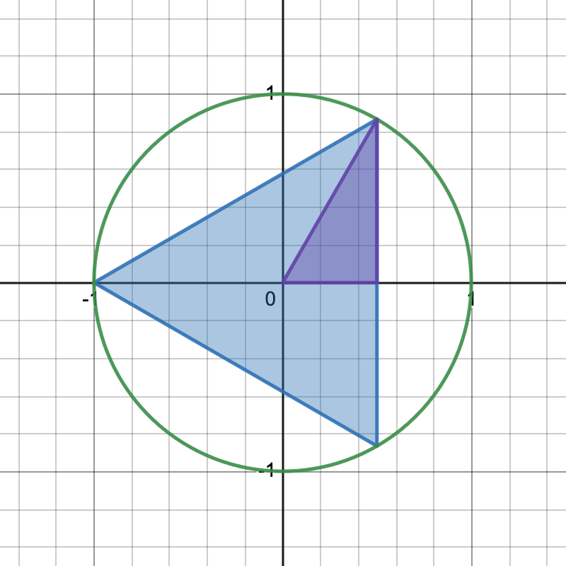
1. What is the area of a regular $n$-gon inscribed in the unit circle?

2. What happens to the area as the number of sides gets bigger and bigger?

A sequence is a special kind of function which has domain equal to the natural numbers $\mathbb{N} = \{1,2,3,\ldots\}$. We say that an interval $(a,b)$ eventually contains a sequence $s(n)$ if there is a number $N$ such that $a < s(n) < b$ for all $n \ge N$. If every interval $(a,b)$ that contains $L$ eventually contains $s(n)$, then we say that $s(n)$ converges to the limit $L$. This can be written as: $$\lim_{n \rightarrow \infty} s(n) = L.$$

We finished by looking at another example of a limit. Galileo was the first person to observe that the distance traveled by an object that is dropped from a great height is roughly $d = 4.9t^2$ meters (when $t$ is the time in seconds after the object was dropped). The average velocity of a falling object is $$v_{\text{average}} = \frac{d(t_2) - d(t_1)}{t_2 - t_1}.$$

3. Use Desmos to find the average velocity over the following time intervals:
   1. $[2,3]$
   2. $[2,2.1]$
   3. $[2,2.01]$
   4. $[2,2.001]$
4. Use the previous answers to estimate the velocity at the instant when the object has been falling for 2 seconds.

These two examples, the area of a circle and the instantaneous velocity of a falling object, are both limits. Next week, we’ll look at how to work systematically with limits.

Week 3 Notes

Mon, Jan 29

Today we defined limits for functions. We say that the limit of $f(x)$ as $x$ approaches $a$ is $L$ and write $$\lim_{x \rightarrow a} f(x) = L$$ if every sequence $x(n)$ that converges to $a$ (but never equals $a$) has $\lim_{n \rightarrow \infty} f(x(n)) = L$.

We looked at two examples on Desmos where a function is not defined but its limit is:

1. $\lim_{x \rightarrow 1} \dfrac{x^3 - 1}{x-1}$.

2. $\lim_{x \rightarrow 0} \dfrac{\sqrt{x^2 + 9} - 3}{x^2}$.

Both of these are examples of hole discontinuities. We also saw three other common types of discontinuities:

3. (Pole discontinuity) $f(x) = \dfrac{1}{x}$ at $x = 0$.

4. (Jump discontinuity) $\operatorname{sign}(x) = \begin{cases} \dfrac{|x|}{x} & \text{ if } x \ne 0 \\ 0 & \text{ if } x = 0 \end{cases}$.

5. (Oscillation discontinuity) $f(x) = \sin(1/x)$ at $x=0$.

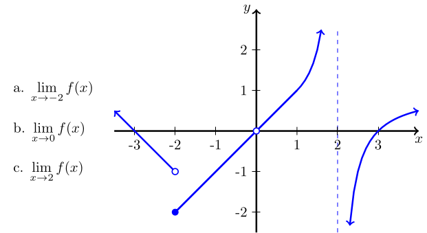
In all three of these cases, the limit at the point of interest does not exist. But there are also one-sided limits which do exist. For example, the one sided limit as $x$ approaches $0$ from above is in example 3 is: $$\lim_{x \rightarrow 0^+} \dfrac{1}{x} = +\infty$$ and the one-sided limit as $x$ approaches $0$ from below in number 4 is: $$\lim_{x \rightarrow 0^-} \operatorname{sign}(x) = -1.$$ You mostly just need an intuitive understanding that a limit is the $y$-value that the graph is heading towards, not the actual $y$-value at the point.

We did the following two examples of finding limits graphically:

6. Two limit examples from Kahn Academy.

We finished by talking about another example of a limit:

$$\lim_{n \rightarrow \infty} (1+r)^n = e^r.$$

Wed, Jan 31

Today we talked about using algebra to find limits. We did the following examples.

1. $\lim_{x \rightarrow -3} \dfrac{x^2 + 3x}{x^2 - x - 12}$. (https://youtu.be/xSlfO2xZDAQ)

2. $\lim_{x \rightarrow 2} \dfrac{2x^2 - 3x + 1}{x^3 + 4}$.

3. $\lim_{x \rightarrow -4} \dfrac{\frac{1}{4} + \frac{1}{x}}{4+x}$. (https://youtu.be/AVOietFdB0c)

4. Find $\lim_{x \rightarrow 5^-} \dfrac{3}{x-5} ~~ \text{ and } ~~ \lim_{x \rightarrow 5^+} \dfrac{3}{x-5}$. (https://youtu.be/bV0RTtywt4g)

At this point, defined continuous functions. A function $f(x)$ is continuous at $x = a$ if $\lim_{x \rightarrow a} f(x) = f(a)$. Intuitively, a function is continuous if you can draw it without lifting your pencil. Most simple functions (including all linear functions and $\sin(x)$ and $\cos(x)$) are continuous at every real number. It turns out that every function constructed from other continuous functions using the operations of addition, subtraction, multiplication, division, powers, and function composition are always continuous at every point in their domains. The only functions you need to worry about are piecewise functions.

5. $\lim_{x \rightarrow 4} f(x)$ where $f(x) = \begin{cases} \frac{x+2}{x-1} & \text{ for } x \le 4 \\ \sqrt{x} & \text{ for } x > 4.\end{cases}$ (https://youtu.be/2xdh0yKopB8)

Fri, Feb 2

Today we went over homework 3.

Week 4 Notes

Mon, Feb 5

We started by talking about continuity.

1. One year I had a job that reimbursed me 50 cents per mile driven, as long as I drove less than 100 miles. For trips of 100 miles or longer, it switched to only reimbursing 30 cents per mile. So the reimbursement $R$ was a piecewise function of the mileage $x$: $$R(x) = \begin{cases} 0.50 x & \text{ if } x < 100 \\ 0.30 x & \text{ otherwise.} \end{cases}$$ What is wrong with this reimbursement function? Hint, what is $R(99)$ vs. $R(100)$?

We also talked about the intermediate value property of continuous functions. If $f(x)$ is continuous on an interval $[a,b]$, and $y$ is between $f(a)$ and $f(b)$, then there is a point $c$ between $a$ and $b$ such that $f(c) = y$.

2. Give an example of an interval $[a,b]$ and a function $f(x)$ that does not have the intermediate value property.

Then we introduced the derivative $f'(a)$ for a function $f(x)$ at a point $x = a$. The derivative is the slope of the tangent line of the function $f(x)$ at the point $(a,f(a))$. The actual definition of the derivative is $$f'(a) = \lim_{x \rightarrow a} \frac{f(x) - f(a)}{x-a}.$$

We calculated some examples.

3. Find the derivative of $f(x) = x$ at any point $a$.

4. Find the derivative of $f(x) = x^2$ at $a = 3$.

5. What is the derivative of $f(x) = |x-2|$ at $a = 2$? Why doesn’t it exist?

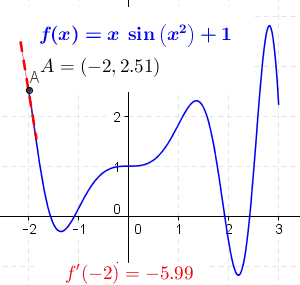
6. Find the derivative of $f(x) = \sqrt{x}$ at $a = 4$. To do this last problem, you need to find $\lim_{x \rightarrow 4} \dfrac{\sqrt{x} - 2}{x- 4}$. (https://youtu.be/8LJC56j9gHA)

Wed, Feb 7

Today we observed that the derivative of $f(x)$ is a function $f'(a)$ that depends on the point $a$ where you found the slope of the tangent line. Another way to write the definition of derivative is: $$f'(x) = \lim_{h \rightarrow 0} \frac{f(x+h) - f(x)}{h}.$$ We also have two different notations for the derivative function. We’ve already seen $f'(x)$. We also use the symbol $\dfrac{d}{dx}$ as a command that literally means “take the derivative of” whatever function comes next. So $f'(x)$ means the same thing as $\dfrac{d}{dx} \, f(x).$ Another notation that we use frequently is to write $\dfrac{dy}{dx}$ to represent the derivative of a function $y = f(x)$. So if we have a function $y = f(x)$, then all of these are the same: $$f'(x) = \dfrac{d}{dx} \, f(x) = \dfrac{dy}{dx}.$$

We used the definition formula above to find

1. $\dfrac{d}{dx} \, x^2$.

2. $\dfrac{d}{dx} \, \dfrac{1}{x}$.

We also looked at how the graph of a derivative $f'(x)$ is related to, but different from, the graph of the original function $f(x)$.

3. Try to graph the derivative of the function shown in this gif:

4. Sketch a rough graph of the derivative of the function below.

We finished by talking about the two meanings of the derivative.

1. The derivative is the slope of the tangent line.
2. The derivative is the instantaneous rate of change.

We looked at this example.

5. A rock falls from a 100 foot cliff with height $h(t) = 100 - 16t^2$ where $t$ is measured in seconds. What is the meaning of the derivative $h'(t)$ in this context, and what are its units?

Fri, Feb 9

Today we introduced the following derivative rules.

1. Linear Function Rule. $\dfrac{d}{dx} [m x + b] = m$.
2. Addition Rule. $\displaystyle\dfrac{d}{dx} \left[f(x) + g(x) \right] = f'(x) + g'(x)$.
3. Constant Multiple Rule. $\dfrac{d}{dx} \left[ c f(x) \right] = c f'(x)$.
4. Power Rule. $\dfrac{d}{dx} x^n = n x^{n-1}$.

We used these rules to solve the following problems.

1. Find $f'(x)$ when $f(x) = x^3 - 5x^2 + 7x - 4$. (https://youtu.be/8Sv6CNuNwqo)

2. Find points on the curve $y = 2x^3 + 3x^2 - 12 x + 1$ where the tangent is horizontal. (https://youtu.be/KxqKelxk3FA)

3. Find the derivatives of $\dfrac{1}{x^2}$, $\sqrt[3]{x^2}$, and $x \sqrt{x}$. Use the exponent rules before you use the power rule.

We also talked about higher derivatives. The second derivative of a function $y = f(x)$ is: $$y'' = \dfrac{d}{dx} \left( \dfrac{d}{dx} \, y \right) = \dfrac{d^2}{dx^2} \, y = \dfrac{d^2 y}{dx^2} = f''(x).$$

We can also take 3rd, 4th, etc. derivatives and they have similar notation.

4. Find the second derivative $y''$ when $y = \dfrac{6}{x^2}$. (https://youtu.be/WC5VYKI807Q)

Week 5 Notes

Mon, Feb 12

In class today, we covered these four derivative rules:

• Derivatives of Sine & Cosine. $$\dfrac{d}{dx} \, \sin x = \cos x ~~~\text{ and }~~~ \dfrac{d}{dx} \, \cos x = -\sin x$$
• Product Rule. $$\dfrac{d}{dx} \, f(x) g(x) = f'(x) g(x) + g'(x) f(x)$$
• Quotient Rule. $$\dfrac{d}{dx} \, \frac{f(x)}{g(x)} = \dfrac{g(x) f'(x) - f(x) g'(x)}{[g(x)]^2} = \frac{\text{Lo}\, \text{DHi} - \text{Hi}\, \text{DLo}}{\text{LoLo}}$$

We did the following examples.

1. $\dfrac{d}{dx} \, x^2 \sin x$ (https://youtu.be/79ngr0Bur38)

2. Let $f(x)$ and $h(x)$ have values in the following table. Find the derivative of $f(x) h(x)$ at $x=3$. (https://youtu.be/SQUSh1LNjIo)

3. $\dfrac{d}{dx} \, x^2 ( x^3 + 4)$ (https://youtu.be/uPCjqfT0Ixg)

4. $\dfrac{d}{dx} \, \dfrac{5x - 3}{x^2+1}$

5. $\dfrac{d}{dx} \, \dfrac{\cos x}{x^2}$ (https://youtu.be/7TXDubwGOSk)

We also gave a proof of the product rule similar to the one in this video.

Wed, Feb 14

Today we focused on examples of derivatives and what they mean.

1. A rock falls from a 100 foot cliff with height $h(t) = 100 - 16t^2$ where $t$ is measured in seconds. What is the velocity of the rock when it hits the ground (i.e., when $h(t) = 0$)? (https://youtu.be/OIo5lfyc8A0)

2. What is the acceleration of the rock?

3. (Exercise 3.4.164) A small town in Ohio commissioned an actuarial firm to conduct a study that modeled the rate of change of the town’s population. The study found that the town’s population (measured in thousands of people) can be modeled by the function $P(t) = -\tfrac{1}{3}t^3 + 64t + 3000$ where $t$ is measured in years.

   1. What is $P'(t)$ and what are its units?

   2. What is $P''(t)$ and what are its units? What does the second derivative tell us about the population.

4. A company sells widgets. The amount of widgets they can sell depends on the price $p$ in dollars. Suppose that quantity sold is $Q(p) = 100 - 4p$.

   1. What is the total revenue $R(p)$?

   2. What does the derivative $R'(p)$ mean?

5. Let $y = \dfrac{x^2 - 1}{x^2 + x + 1}$. Find the tangent line at the point $(1,0)$. (https://youtu.be/8p7QGLzOynI)

6. Let $f(x) = 5-x^2$. Find the tangent line to $f(x)$ when $x= 2$. Where does that tangent line intersect they $x$-axis?

Week 6 Notes

Mon, Feb 19

Today we covered the derivatives of trigonometric functions in more detail. We started with this limit problem.

1. Find the limit $\lim_{h \rightarrow 0} \dfrac{1 - \cos h}{\sin h}$. Hint: First multiply the top & bottom by $1 + \cos h$.

Then we applied that limit to prove the two fundamental limits of trigonometry

$$\lim_{h \rightarrow 0} \frac{\sin h}{h} = 1 \text{ and } \lim_{h \rightarrow 0} \frac{\cos h - 1}{h} = 0.$$

Then we used the angle addition formula for $\sin(x+h)$ to prove that $\dfrac{d}{dx} \sin x = \cos x$. Then we solved the following problems.

2. Find the derivatives of $\tan x$ and $\sec x$.

3. Find the derivative of $y = 2x \cos x - 2 \sin x$. (https://youtu.be/tXc8A3VpNOI)

4. Find the derivative of $y = x \sin x$.

We finished by looking at the graph of $y = \sin (2 x)$. This is a wave that oscillates twice as fast as the regular $\sin x$. So intuitively, its tangent lines should be twice as steep. It turns out that they are because of the chain rule which is a rule for taking the derivative of functions when they are composed together.

Wed, Feb 21

Today covered the chain rule in more detail.

1. $\dfrac{d}{dx} \sqrt{1-x^2}$.

2. Compare these two derivatives $\dfrac{d}{dx} \sin^2 x$ versus $\dfrac{d}{dx} \sin(x^2)$.

3. We didn’t do this one in class, but it is a good exercise: Use Leibniz notation to find the derivative of $y = \sqrt{5x+1}$. (https://youtu.be/Ur_kdKXnZPo)

4. Find the derivative of $f(x) = \cos^2 8x$. (https://youtu.be/TlE8bXB53Zw)

5. Find $\dfrac{d}{dx} \sqrt{\tan 5x}$. (https://youtu.be/S62sK5XoRQo)

6. Find the equation for the tangent line to the function $y = \sqrt{25-x^2}$ at the point $(3,4)$.

Fri, Feb 23

Today we talked about the chain rule some more. We did the following examples.

1. Find the derivative of $y = \left( \dfrac{x-1}{2x+1} \right)^7$. (https://youtu.be/ed5pQoqHXeU)

2. Suppose that the crime rate $C(p)$ in a city is a function of the population $p$. The population $p=p(t)$ is a function of time $t$ in years. Suppose that the city’s population is currently 300,000 at $t=0$. If $p'(0) = 5,000$ people per year and $C'(300,000) = 0.4$ crimes per person, then estimate the rate of change in crime this year.

3. Let $\operatorname{sind}$ be the sine function for angles measured in degrees. So for example, $\operatorname{sind}(90^\circ) = 1$. What is the derivative of $\operatorname{sind} x$? Hint: $\operatorname{sind} x = \sin( \tfrac{\pi}{180} x)$.

4. Find $\dfrac{d^2}{dx^2} \tan (x^2)$.

Week 7 Notes

Mon, Feb 26

To we introduced implicit equations and implicit differentiation. Implicit equations involving $x$ and $y$ are sometimes called implicit functions, but they aren’t really functions because one $x$ value can correspond to multiple $y$ values. But if we act like $y$ is a function of $x$ and use the chain rule each time we see a $y$ in the equation, we can still find the derivative $y'$ which is still the slope of the tangent line. We started with this example.

1. Find the slope of the tangent line at the point $(3,4)$ on the circle defined by $x^2 + y^2 = 25$.

2. Find $y'$ for any point on the parabola $y^2 = x$.

3. Find $\dfrac{dy}{dx}$ when $\sin(x+y) = -y^3$.

4. Consider the closed curve defined by the equation $$x^2 + 2x +y^4 + 4y = 5.$$ Find the coordinates of the two points on the curve where the tangent line is vertical. (https://youtu.be/-jcVn0yCJ6E)

We didn’t get to this last example, except to mention its name, but I’ll mentioned it now, and hopefully get to it next time.

1. The folium of Descartes is a curve defined by the implicit formula $$x^3 + y^3 = 6xy.$$
   1. Find the slope of the tangent line to the folium of Descartes at $(3,3)$.
   2. Where is the slope of the tangent line horizontal? (https://youtu.be/mtYbKR2DMuI)

Wed, Feb 28

We started with some more examples of implicit differentiation.

1. The folium of Descartes is a curve defined by the implicit formula $$x^3 + y^3 = 6xy.$$
   1. Find the slope of the tangent line to the folium of Descartes at $(3,3)$.
   2. Where is the slope of the tangent line horizontal? (https://youtu.be/mtYbKR2DMuI)
2. Find the second derivative $\dfrac{d^2 y}{dx^2}$ when $y^2 - x^2 = 4$. (https://youtu.be/oPijG5Bfemg)

Then we introduced an application of implicit differentiation called related rates with the following example. First note that an object moving on the xy-plane has two components of velocity:

• Horizontal velocity $\dfrac{dx}{dt}$,
• Verical velocity $\dfrac{dy}{dt}$.

If we know one of these velocities, we can use implicit differentiation to find the other.

3. Suppose that a car is driving around a circular race track with a 1 kilometer radius. The equation of the race track is $$x^2 + y^2 = 1.$$ If the car has horizontal velocity $\dfrac{dx}{dt} = -50 \text{ km/hr}$, when its position is $\left( \tfrac{\sqrt{3}}{2}, \tfrac{1}{2} \right)$, then what is its vertical velocity at that instant?

Fri, Mar 1

Today we talked about related rates. We did these examples.

1. A pebble dropped into a pond makes circular ripples. The radius of the ripples increases at a rate of 1 cm/sec. Find how fast the area is increasing when the radius is 3 cm. (https://youtu.be/kQF9pOqmS0U)

2. A 10 foot long ladder leans against a wall. Suppose the bottom of the ladder is sliding away from the wall at a rate of 2 ft/sec when the base of the ladder is 6 ft. away from the wall. How fast is the top of the ladder sliding down at that instant? (https://youtu.be/p_QyOi2MbFQ)

3. A camera is rotating to track a rocket launched vertically from a platform that is 3,000 ft from the camera. If the rocket’s velocity is 1,000 ft/sec, how fast is the camera angle changing (in radians/sec) when the rocket is 4,000 feet up?

Here is one more example that we didn’t have time for in class:

4. A 6 foot tall man is walking away from a 15 foot tall streetlight at 5 feet/sec. How fast is the man’s shadow growing when he is 40 feet from the base of the light? (https://youtu.be/xe6MAJB7CPI)

Week 8 Notes

Mon, Mar 4

We’ve already talked about tangent lines, but a tangent line at a point $(a, f(a))$ on the graph of a function $y = f(x)$ is the best linear approximation function for $f(x)$ near $x = a$ (also known as the linearization. It is important enough that I have included this formula $$f(x) \approx f(a) + f'(a) (x - a)$$ on the formula sheet. Sometimes we use $L(x) = f(a) + f'(a) (x-a)$ to denote this linear approximation function.

1. Find a linear approximation for the function $f(x) = \sqrt{x}$ near $a = 4$, then use it to estimate $\sqrt{4.36}$. (https://youtu.be/u7dhn-hBHzQ)

2. Find the linearization of $f(x) = \sqrt[4]{x}$ at $x = 625$. Use this to estimate $\sqrt[4]{610}$. (https://youtu.be/oYSyaM9wB9U)

3. Find the linearization of $f(x) = \cos x$ at $a = \tfrac{\pi}{2}$. (https://youtu.be/l8PFsYI3bzw)

4. Suppose I drive 360 miles, and then need to fill up my car with gas. If it takes 10.5 gallons, I’d like to estimate how many miles per gallon my car got on that last tank of gas. So I have to calculate $\dfrac{360}{10.5}$, but that is too hard to do without a calculator. Instead, I can use a linearization of the function $f(x) = \dfrac{360}{x}$ at the point $a = 10$ to try to get a good estimate.
   

Wed, Mar 6

Today we introduced differential notation. For a function $y = f(x)$ and two $x$-values $x_0$ and $x_1$, we can talk about the change in x and the change in y:

$$\Delta x = x_1 - x_0 \text{ and } \Delta y = f(x_1) - f(x_0).$$

If we use the tangent line $L(x)$ at $x= x_0$ instead of the function $f(x)$ to find the change in $y$, then we get what are called differentials:

$$d x = x_1 - x_0 \text{ and } dy = f'(x_0) dx.$$

Intuitively, $dx$ and $\Delta x$ are two different notations for the exact same thing. But $dy$ and $\Delta y$ are not the same. The differential $dy$ is the change in $y$ using the tangent line while $\Delta y$ is the change in $y$ using the function $f(x)$.

1. Find the differential of $y = x^4 + 6$ at $x=-1$ when $dx = 0.1$ (https://youtu.be/4qqNe_hfoz8)

2. Find the differential of $y = \sin(5x^2)$. (https://youtu.be/CGDeNaR0LYk)

3. Ignoring air resistance, then range of a canonball launched with angle of elevation $\theta$ in a large flat field is $R = \dfrac{v_0^2}{g} \sin(2\theta)$.

   1. How far will the canonball go if $v_0 = 147$ m/s and $\theta = \pi/12$?
   2. How much farther would it go if we increase $\theta$ by $0.1$ radians?

4. The (average) radius of the Earth is approximately $r= 3959$ miles. The radius is actually a little bit lower than that. There is error in the number $r$ which can be represented by saying that $dr = 0.2$. If we use the radius to compute the surface area using the formula $S = 4\pi r^2$, how much error $dA$ might there be in our calculated answer? (https://youtu.be/CGDeNaR0LYk?t=185)

The answer to the last exercise seems big ($dS = 8\pi (3959) (0.2) = 19,900$ square miles). But relative to the surface area of the Earth, it actually isn’t that big. So when working with differentials to estimate measurement error, we often calculate the relative error which is $$\text{Relative error} = \frac{\Delta y}{y} \approx \frac{dy}{y}.$$

5. Find the approximate relative error in our calculation of the Earth’s surface area.

Fri, Mar 8

Today we talked about how to find the absolute maximum and minimum (also known as the global maximum/minimum) of a function on a closed interval $[a,b]$. For a continuous function $f(x)$ on an interval, there is always an absolute max (and min) and it will always occur at either an endpoint of the interval or at a critical point which is a point $c$ where $f'(c) = 0$ or $f'(c)$ does not exist.

1. Find the absolute maximum and minimum of $f(x) = x^4 - 2x^3$ on the interval $[-2,2]$. (https://youtu.be/ADvCJh9seIY)

2. Find the absolute maximum and minimum of $f(x) = \sin x + \cos x$ on the interval $[0,\tfrac{\pi}{3}]$. (https://youtu.be/cV1tpeY5mE4)

3. Find the absolute maximum and minimum of $y = 2x - 3x^{2/3}$ on $[-1,3]$.

Here is one more example that we did not have time for in class.

4. Find the absolute maximum and minimum of $f(x) = 2x^3 - 6x - 1$ on $[-3,2]$. (https://www.youtube.com/watch?v=ADvCJh9seIY&t=358s)

Week 9 Notes

Mon, Mar 18

1. Find the absolute maximum and minimum of $f(x) = 2x^3 - 6x - 1$ on $[-3,2]$. (https://www.youtube.com/watch?v=ADvCJh9seIY&t=358s)

2. Give an example of a discontinous function with no absolute max or min on the interval $[1,3]$.

3. Given an example of a continous function with no absolute max or min on the interval $(1,3)$.

4. Find the absolute maximum and minimum of $f(x) = \sin x + \sin^2 x$ on $[0, 2\pi]$.

5. Find the critical x-values of $g(\theta) = 4 \theta - \tan \theta$. (https://youtu.be/XJwpmKyaG3A)

6. Find the absolute max and min for $g(\theta)$ on $[0,1.5]$ (okay to use a calculator).

Wed, Mar 20

We started with this warm-up problem.

1. Find $y'$ if $\sec(xy) = y$.

Then we proved some theorems. We started with this theorem:

To prove Rolle’s theorem, we answered these questions:

1. How do we know that $f$ has an absolute max and an absolute min on $[a,b]$?

2. What would happen if the absolute max and absolute min both happen at the endpoints? What would that mean about $f$?

3. What would happen if either the absolute max or absolute min occurs inside $(a,b)$? What would that mean about the point $c$ in $(a,b)$ where the absolute max or min occurs?

After proving Rolle’s theorem, we introduced the mean value theorem (MVT for short).

Intuitively this makes sense. It says that the average rate of change over an interval is equal to the instantaneous rate of change at at least one point inside the interval. We talked about the example of drive 100 miles in just 1 hour on a highway. How can you tell that your car’s speedometer actually hit 100 mph exactly?

4. To prove the mean value theorem, let $L(x)$ be the linear function passing through the points $(a, f(a))$ and $(b, f(b))$.
   1. What is the slope of $L(x)$?
   2. What does Rolle’s theorem say about the function $f(x) - L(x)$ on $[a,b]$?

We finished by talking about some applications of the MVT.

5. If $f'(x) = 0$ for every $x$ in $[a,b]$, what does the mean value theorem say about $f(b)$ and $f(a)$?

6. If $f'(x) > 0$ for every $x$ in $[a,b]$, what does the mean value theorem say about $f(b)$ and $f(a)$ when $b > a$?

Week 10 Notes

Mon, Mar 25

Today we talked about using the first derivative to find the intervals of increase and decrease of a function. We did the following examples.

1. $f(x) = 2x^3 + 18x^2 + 30x + 3$ (https://youtu.be/jB451pFTi6c)

2. $g(x) = x^4 - x^5$ (https://youtu.be/x09FpMmGB4A)

3. $f(x) = \dfrac{x^2 - 2}{2x+3}$ (https://youtu.be/AI1JJXY4Aj0)

4. $y = (x^2 - 4)^{2/3}$

Wed, Mar 27

We started with this example where we found intervals of increase and decrease as well as local max & mins.

1. $g(x) = x + 2 \sin x$ on $[0,2\pi]$ (https://youtu.be/BLn2B0azut8?t=79)

Then introduced the notion of concavity. A function $f(x)$ is concave down at $x = a$ if $f(x)$ is below the tangent line $L(x)$ for all $x$ near $a$. The function is concave up if $f(x)$ is greater than $L(x)$ for all $x$ close to $a$. It turns out that a function $f$ is concave up exactly when the second derivative $f''(x)$ is positive and concave down when $f''(x)$ is negative. A point where the concavity changes from positive to negative or vice versa is called an inflection point.

We used the second derivative to find the intervals of concavity (intervals where the function is concave up or concave down) for these functions, and we also found the inflection points.

2. $f(x) = 2x^3 + 6x^2 - 5x + 1$ (https://youtu.be/AeMWC8TTMZU)

3. $y = \dfrac{x}{x^2 + 1}$ (https://youtu.be/EggCllDCuw8)

Fri, Mar 29

Today we applied the techniques we’ve learned to solve optimization word problems. We did these examples.

1. A farmer wants to fence off a rectangular plot of land along the side of a long straight river. He has a total of 2400 feet of fence. How large of and area can he fence off? (https://youtu.be/gt4Qtp0Wxtk)

2. A cylindrical can must hold 1 liter (1000 cubic centimeters) of oil. What dimensions (height and radius) minimize the surface area of the can? (https://youtu.be/e0Fgyca6WCw) Note: I made a mistake when I solved this in class and forgot a square at one point. Sorry about that!

We also talked about using the first derivatives and the intervals of increase/decrease to double check that a critical point is a max or a min (the first derivative test) and how to check whether a critical point is a max or min by checking the second derivative at that point (the second derivative test).

Here are some other examples that we didn’t have time for today.

1. A rectangular piece of cardboard is 20 inches by 30 inches. If we cut a square from each corner of the cardboard and fold up the sides to make a box, how big should the squares be in order to maximize the volume? (https://youtu.be/MC0tq6fNRwU and https://youtu.be/cRboY08YG8g)

2. A cone is made from a circular piece of paper (with radius $R$) by cutting out a slice and bringing the two sides of the slice together. Find the height of the cone that maximizes the volume. (https://youtu.be/ZNoJThDRBcw)

3. Find the point on the parabola $x = \tfrac{1}{2}y^2$ that is closest to the point $(1,4)$. (https://youtu.be/ZZYf4hzluKw)

Week 11 Notes

Wed, Apr 3

We started with this optimization example which we did not get to last time.

1. Find the point on the parabola $x = \tfrac{1}{2}y^2$ that is closest to the point $(1,4)$. (https://youtu.be/ZZYf4hzluKw)

Then we introduced limits as $x$ approaches infinity. The key idea when taking the limit of a polynomial expression as $x \rightarrow \pm \infty$ is to factor out the highest power of $x$. We used that idea on all of these examples:

1. $\lim_{x \rightarrow -\infty} x^4 + 100 x^3$

2. $\lim_{x \rightarrow \infty} \dfrac{10x^3 + x^2 - 5}{8 - 4x - 4x^3}$ (https://youtu.be/-UQBxnNZ8-Q)

3. Find $\lim_{x \rightarrow \infty} f(x)$ and $\lim_{x \rightarrow -\infty} f(x)$ when $f(x) = \dfrac{-2x + 1}{\sqrt{9x^2 - 16}}$ (https://youtu.be/qNhV2S2whyw)

Here are a few more examples we didn’t have time for in class.

1. $\lim_{x \rightarrow \infty} \dfrac{2x+3}{x^2+4}$ (https://youtu.be/eB829NO82ew)

2. $\lim_{x \rightarrow \infty} \dfrac{5x - 7}{3x+4}$ (https://youtu.be/eB829NO82ew)

Fri, Apr 5

Today we introduced L’Hospital’s rule which is a fast way to calculate limits when you have an indeterminant form $\tfrac{0}{0}$ or $\tfrac{\infty}{\infty}$. We did these examples.

1. $\displaystyle \lim_{x \rightarrow 0} \dfrac{\sin x}{x}$. (https://youtu.be/PdSzruR5OeE)

2. $\lim_{x \rightarrow \infty} \dfrac{x^2+x}{2x^2}$.

3. $\lim_{x \rightarrow 0} \dfrac{(1+x)^n - 1}{x}$.

4. $\displaystyle \lim_{x \rightarrow 5^+} \dfrac{x}{x-5}$. (You can’t use L’Hospital’s rule here! Why not?)

5. $\displaystyle \lim_{x \rightarrow \infty} \dfrac{3x^{8}-4x^{7}+3x^{4}}{2x^{7}+5x^{5}-3x}$ (Hint: The key to this one is to factor out the highest power of $x$ in the numerator & denominator).

6. $\lim_{x \rightarrow \pi} \dfrac{\cos x + 1}{x - \pi}$.

Week 12 Notes

Mon, Apr 8

Today we introduced antiderivatives also known as indefinite integrals. To find the antiderivative of a function $f(x)$, you just need to find a function $F(x)$ that has $f(x)$ as its derivative. We started with this example:

1. $\int 2x \, dx$ (https://youtu.be/MMv-027KEqU)

We introduced these rules for integrals:

We applied those rules to these examples:

2. $\int x^5 \, dx$

3. $\int \sqrt{x} \, dx.$

4. $\int 9x^{11} + 4x^6 - 9x^2 - 3 \, dx$ (https://youtu.be/RMtjkFUjem4)

5. $\int - \dfrac{7}{x^3} \, dx$ (https://youtu.be/1ZtwjxzbU68?t=54)

6. $\int \dfrac{\sqrt{x} - 5x}{x^3} \, dx$

We also looked at antiderivatives of trig functions

7. $\int \cos x \, dx$

8. $\int \sec x \tan x \, dx$

9. Find the antiderivative of $f(\theta) = 2 \sin \theta - \sec^2 \theta$. (https://youtu.be/EpH4rN93ftc)

We finished by discussing how you can use antiderivatives to find the velocity and position of a falling object if you know its acceleration by integrating:

10. Find the velocity $v(t)$ of a falling object by integrating $\int -9.8 \, dt$.

11. Find the position $s(t)$ by integrating $\int -9.8 t + v_0 \, dt$.

Wed, Apr 10

Today we looked at more examples of antiderivatives. We started with a theorem.

We proved this theorem by observing that the function $\operatorname{gap}(x) = G(x) - F(x)$ has derivative equal to zero everywhere. Therefore there cannot be two different points $a, b$ such that $\operatorname{gap}(a)$ is different than $\operatorname{gap}(b)$, otherwise, the MVT would imply that $\operatorname{gap}'$ would be non-zero somewhere on the interval from $[a,b]$. Therefore the function $\operatorname{gap}(x)$ is constant.

After proving this theorem, we talked about initial value problems. This is when you are given the derivative of a function and the value of the function at one point and are able to use integration to find the exact value of the function. We did the following examples.

1. Solve $\dfrac{dy}{dx} = 6x - 3$ with initial condition $y(0) = 4$. (https://youtu.be/kwGukY_2qWQ)

2. Solve $\dfrac{dy}{dx} = -4 \cos(x-3)$ with initial condition $y(3) = -5$. (https://youtu.be/gw3jd921Zzc)

3. Solve $\dfrac{ds}{dt} = \cos t + \sin t$ given that $s(\pi) = 1$. (https://youtu.be/tXR__A_jkxE)

4. Find $f(x)$ if $f'(x) = x^2$ and the graph of $f(x)$ passes through $(3,14)$.

5. Suppose that $f''(x) = 20x^3 + 12x^2 + 4$, $f(0) = 8$ and $f(1) = 5$. (https://youtu.be/ETixs3tYAXE)

6. The acceleration of gravity is $-32$ feet per second squared. If a rock is thrown upwards from a platform located 20 feet above the ground with initial velocity 30 feet per second, find formulas for the height and velocity of the rock as functions of time.

Fri, Apr 12

Today we introduced Riemann sums as a way to approximate the area under a curve. We started with the curve $y = 2x-x^2$ as an example.

The formula for finding a Riemann sum approximation (using right endpoints) is

1. Use Desmos to approximate the area under $f(x) = 2x - x^2$ on the interval $[0,2]$ with $N = 100$ rectangles. (https://www.desmos.com/calculator/j5is4fibzg)

We also reviewed summation notation. If you aren’t familiar, here is a good explanation:

2. $\sum_{n=1}^3 2n+3$. (https://youtu.be/lQZY4pD8X6I)

We did the following in class:

3. $\sum_{i = 1}^5 i$.

4. $\sum_{i = 1}^{100} i$. (We derived the formula $\sum_{i = 1}^N i = \tfrac{1}{2}N(N+1).)$

5. $\sum_{n = 1}^{100} 4n+5$. (https://youtu.be/xavgv1m9feE?t=298)

Here is another example we didn’t do:

6. $\sum_{n = 1}^5 n^2$. (https://youtu.be/xavgv1m9feE)

Week 13 Notes

Mon, Apr 15

Today we introduced the definite integral which is defined as the limit of the Riemann sum as the number of rectangles $N$ approaches infinity: $$\int_a^b f(x) \, dx = \lim_{N \rightarrow \infty} \sum_{n = 1}^N f(x_n) \Delta x.$$ A function is integrable on an interval $[a,b]$ if this limit exists.

We approximated the following definite integrals using Desmos to calculate the Riemann sum:

1. $\int_0^\pi \sin x \, dx$ (https://youtu.be/JgGXnBaI8-E)

2. $\int_2^5 \dfrac{1}{x} \, dx$

Because the definite integral is the area of the curve, sometimes you can find the answer without calculus if you recognize the shape:

3. $\int_2^5 x \, dx$

4. $\int_{-1}^1 \sqrt{1-x^2} \, dx$

Another important concept is that area beneath the x-axis counts as negative area. We did this example by looking at the shapes and finding the positive and negative area.

5. $\int_0^3 1 - x \, dx$.

Definite integrals have these important properties:

We did the following additional examples.

6. Suppose that $\int_3^6 g(x) \, dx = -8$ and $\int_3^9 g(x) \, dx = 5$. Find $\int_6^9 g(x) \, dx$. (https://youtu.be/QcHz3h81U-s?t=305)

7. Suppose that $\int_{-1}^3 f(x) \,dx = -2$ and $\int_{-1}^3 g(x) = 5$, then find $\int_{-1}^3 3f(x) - 2g(x) \, dx.$ (https://youtu.be/TqMxlzZiKg4)

Wed, Apr 17

Today we talked about

We explained why this theorem makes sense by changing the letter $b$ to a letter $t$ to emphasize that the formula above is a function of the upper bound in the integral. And we showed that the derivative of the area function $A(t)$ is $f(t)$, so it makes sense that you can use the antiderivative of $f(x)$ to get the area.

We did these examples in class using the Fundamental Theorem of Calculus to evaluate the definite integrals.

1. $\int_0^\pi \sin x \, dx$

2. $\int_1^4 2x^2 - x \, dx$ (https://youtu.be/xo9jxrVGnnY)

3. $\int_0^{\pi/4} \sec^2 t \, dt$ (https://youtu.be/-Hm7w1BqVhA)

4. $\int_1^4 3 \sqrt{x} \, dx$

Just like with derivatives, it is important to understand the meaning of the definite integral.

5. If a particle has velocity $v(t) = 5 - t$, then what is its net change in position from time $t=0$ until time $t=10$? (https://youtu.be/Sy_7PkoTCtA)

6. Water flows out of a tank at a rate $r(t) = 200 - 4t$ liters per minute. Find the amount of water flows out of the tank in the first 10 minutes? (https://youtu.be/66L46J4rxIA)

Week 14 Notes

Mon, Apr 22

Today we looked at more examples of definite integrals and we also defined:

1. Find the average value of $f(x) = x^2 + 1$ on the interval $[0,3]$. (https://youtu.be/0rzL08BHr5c)

We did a few extra problems to see some of the ideas that come up working with definite integrals.

2. $\int_{-1}^2 |4x-3| \, dx$ (https://youtu.be/S5zFfQODQOo)

3. $\dfrac{d}{dx} \int_x^3 \sqrt{|\cos t|} \, dt$ (https://youtu.be/TqGCNNlx6pU) Hint: The key for this problem is to skip the work of finding the antiderivative of $\sqrt{|\cos t|}$. Just use the notation $F(t)$ to represent the antiderivatve temporarily.

We finished by introducing an integration technique called u-substitution which lets you undo a chain rule.

4. $\int 2x \sin (x^2) \, dx$ (https://youtu.be/VPX3dcdWdRM)

Wed, Apr 24

Today we went into more depth about the u-substitution method. We did the following examples.

1. $\int x^2 \cos(x^3) \, dx$ (https://youtu.be/kf2sskrphL0)

2. $\int \sin(2x) \, dx$

3. $\int (5x)^2 \, dx$ (Hint: you don’t have to use substitution for this one, but substitution will work too.)

There is a shortcut for the last two integrals since the derivative of the inside is just a constant. When the derivative of the inside is just a constant, you can use the reverse chain rule: integrate the outside function, leave the inside alone, then divide by the derivative of the inside. Be careful, that does not work if the derivative of the inside is not a constant! We applied the reverse chain rule to

4. $\displaystyle\int \cos (2x) \, dx$

We finished with a couple more complicated u-substitution examples.

5. $\displaystyle\int \dfrac{x^3}{(2+x^4)^2} \, dx$ (https://youtu.be/sdYdnpYn-1o?t=459)

6. $\displaystyle\int \cos (3x) \sin^2 (3x) \, dx$ (https://youtu.be/0zv_4Y9odAQ)