
| Day | Section | Topic |
|---|---|---|
| Mon, Aug 26 | 1.1 | Definitions and algebraic properties |
| Wed, Aug 28 | 1.2 | From algebra to geometry and back |
| Fri, Aug 30 | 1.3 | Geometry of complex numbers |
Today we introduced the complex numbers which are a field. We defined the real and imaginary parts of a complex number and also the absolute value and argument of a complex number. We did the following examples.
Find the real and imaginary parts of by rationalizing the denominator.
Factor the polynomial .
The polynomial is irreducible over , but not over . Show this by factoring it over .
Later in the course we will use complex analysis to prove one of most important theorems in algebra:
The Fundamental Theorem of Algebra. Every polynomial with coefficients in factors into a product of linear expressions of the form where .
We finished with a discussion of the polar form of a complex number.
Following Beck et. al., we will define Later, when we define the complex exponential function, we will revisit this definition. For now, we will do some calculations that suggest the definition is a good one.
Use the angle addition formulas to show that
Simplify .
Calculate . Hint: Use the definition of and treat like any other constant.
What is ?
What is ?
Explain why makes sense in the context of the velocity of a point moving counterclockwise along the unit circle.
After introducing , we discussed the n-th roots of unity which are the complex numbers such that . They are given by the formula
Find the 3rd roots of 8.
Find the 3rd roots of .
We finished with a discussion of square and cube roots of complex numbers and how they relate to roots of unity. We also defined the complex conjugate of to be .
We reviewed some of the useful formulas involving complex conjugates including the following:
and
and
We also introduced and proved the triangle inequality for complex numbers
Use the triangle inequality to prove the reverse triangle inequality by introducing a substitution .
If , prove that
A convex combination of is any point The set of all convex combinations of and is a line segment connecting to , and the formula for the convex combinations is a parametric formula for the line segment. If you allow any , then you get an affine combination of and . The set of all affine combinations of and is line passing through and .
| Day | Section | Topic |
|---|---|---|
| Mon, Sep 2 | Labor Day, no class | |
| Wed, Sep 4 | 1.4 | Elementary topology of the plane |
| Fri, Sep 6 | 1.4 | Elementary topology of the plane - con’d |
Let denote the open disk of radius around . We used to define interior and boundary points for a subset of . We proved the following trichotomy result
Theorem. If and , then exactly one of the following holds.
We also defined open and closed sets, and proved the following theorem.
Theorem. A set is closed if and only if its complement is open.
We also defined bounded sets. We finished by talking about paths which are continuous functions . The range of a path is a subset of called a curve (note that not all books follow this terminology). We defined the derivative of a path, and discussed how to define a smooth path so that it matches our intuition for a curve with no sharp turns.
A path is simple if for all , except possibly at the endpoints and . Intuitively, a path is simple if it cannot cross itself, except possibly at the endpoints. A path is closed if .
A set is path connected if for any , there is a (continuous) path such that and . The following theorem seems obvious, but it is actually famously tricky to prove (see https://en.wikipedia.org/wiki/Jordan_curve_theorem).
The Jordan Curve Theorem. The complement of the range of a simple closed curve in consists of two disjoint open path connected sets, one of which (the inside) is bounded and the other (the outside) is not bounded.
A sequence is a function . We use the notation to mean the same thing as for sequences. A sequence converges to if for every , there is an such that for every . Intuitively, this means that for every open disk around , there can only be a finite number of such that is not in the disk. When a sequence converges, the number it converges to is called its limit.
If we don’t know the limit of a sequence, we can still use Cauchy’s criterion to show that it must converge. A Cauchy sequence is a sequence such that for every , there exists such that whenever .
Theorem (Cauchy’s Criterion). If is a Cauchy sequence, then it converges to some limit in .
We talked about how the Cauchy criterion applies to sequences of real numbers and the complex numbers, in fact the property that Cauchy sequences converge in a set is known as completeness and it is one of the defining properties of the real numbers.
We used completeness to prove the following theorem about real number sequence:
Theorem (Monontone convergence). If is a sequence of real numbers that is monotone (non-decreasing) and bounded, then it converges.
We ran out of time, but a related application of completeness is the following result.
Theorem. If and are both nonempty sets, then has at least one boundary point.
| Day | Section | Topic |
|---|---|---|
| Mon, Sep 9 | 7.1 | Sequences and completeness |
| Wed, Sep 11 | 7.2 | Series |
| Fri, Sep 13 |
The complex numbers are a metric space because they have a distance function that satisfies the following properties for all :
It helps when working with absolute values in to remember that is the distance between and . We didn’t have time for a proof of the last theorem from Friday, so we worked through a proof using the fact that is a complete metric space today. Recall that complete means that all Cauchy sequences converge. We proved the theorem by proving the following claims:
Any line segment that connects a point in to a point in contains a line segment that is half as long and also connects a point in to a point in .
The midpoints of the line segments above form a Cauchy sequence.
The limit of the midpoints is a boundary point of .
This proof definitely doesn’t work without assuming completeness. For example, if , then has no boundary points in . After discussing that example, we talked about infinite series.
A series of complex numbers converges if its sequence of partial sums converges. It helps to know some example infinite series, so we talked about these three:
Zeno’s series .
Grandi’s series .
Harmonic series .
Then we reviewed geometric series which are series of the form where is the first term and is the common ratio. We proved:
Theorem. A geometric series converges if and only if , and in that case
Class was canceled since I was out with COVID.
| Day | Section | Topic |
|---|---|---|
| Mon, Sep 16 | 2.1 | Limits and continuity |
| Wed, Sep 18 | 2.2 | Differentiability and holomorphicity |
| Fri, Sep 20 | 2.2 | The Cauchy-Riemann equations |
Today we reviewed the questions from the infinite series workshop. Then we talked about functions . We defined limits of functions several ways, and we did the following examples.
.
Use the definition of limits to prove that if then .
Consider We can use the fact that to make the top as small as we want. We just need to make sure that the bottom doesn’t get close to zero at the same time. The trick is to use the triangle inequality to show that when ,
Use the sequential definition of limits to prove the product rule for limits, i.e., .
We introduced the complex derivative for functions :
What does it mean for a function to be differentiable? For functions , we say that is differentiable at a vector if there is a matrix (called the Jacobian) such that more specifically, The expression is an affine linear approximation of near .
A complex function can be thought of as a real function , and corresponds to the Jacobian matrix
Observe that if , then . Find the Jacobian of the function and show that it corresponds to the complex number .
Show that the function is not complex differentiable. Explain why that makes sense, even though the corresponding map on , , does have a Jacobian matrix.
We introduced the Cauchy-Riemann equations.
Theorem. Suppose is complex differentiable at , and . Then satisfies the Cauchy-Riemann equations Conversely, if and the partial derivatives of and are continuous in a disk around and satisfy the Cauchy-Riemann equations, then is complex differentiable at .
This is Exercise 2.19 in the book: Define if is on either purely real or purely imaginary, and otherwise. Show that satisfies the Cauchy–Riemann equations at , yet is not differentiable at . Why doesn’t this contradict the theorem about a complex function being complex differentiable if and only if it satisfies the Cauchy-Riemann equations?
We say that a function that is complex differentiable in an open disk around is holomorphic at .
Then we talked about smooth paths which are paths that are differentiable. If is a smooth path in and is holomorphic at every point on the curve, then the chain rule holds and says that
Idea. Notice that the angle of the tangent vector gets rotated by the argument of . If two different smooth curves both intersect at a point , and is holomorphic at , then since their tangent vectors are both rotated by the same angle, the angle between the two tangent vectors stays the same. This implies that holomorphic maps are conformal, that is they preserve angles between curves.
We also looked at the function on the complex grapher and saw that it was also conformal.
| Day | Section | Topic |
|---|---|---|
| Mon, Sep 23 | 3.4 | Exponential and trigonometric functions |
| Wed, Sep 25 | 3.5 | Logarithms and complex exponentials |
| Fri, Sep 27 | 3.1 | Möbius transforms |
We started by reviewing the properties of the exponential function including its algebraic properties, domain, range and that it is periodic with period . Then we introduced the complex natural logarithm which is the inverse of . There is one problem with defining the inverse: is an -to-1 function, every has infinitely many pre-images. So we have two options:
denotes the multivalued inverse of . It has the form where is the multivalued argument function.
is the principal branch of . It is a single valued function of the form where is the single valued principal branch of the argument function that takes values in .
We did the following exercises.
Calculate .
If where , then . Calculate the Cauchy-Riemann equations for to verify that is complex differentiable when (in fact it is complex differentiable everywhere except at its branch cut ). What is the derivative of ?
We looked at the Cauchy-Riemann equations for again. We also did the following.
We introduced principle values of a complex power for any , with . We calculated the following examples.
Find all other values of in addition to the principal value.
Find all solutions of the equation .
We finished by talking about the reciprocal map . We looked at how it appears to transform lines & circles into lines and circles. We’ll look at why next time.
We started by proving this theorem about the reciprocal map.
Theorem. Let . Then transforms lines and circles to lines in circles.
The key to the proof is the fact that the solution of the algebraic equation (with real coefficients) is a circle (possibly degenerate to a point or ) if , and it is a line if .
It helps to think of the reciprocal map as a bijection (1-to-1 and onto map) from . We define We call the extended complex plane.
The reciprocal map is a special case of an important family of bijections on called Möbius transforms. A Möbius transform (also known as a Linear Fractional Transform) is a map where satisfy . We proved the following facts.
A Möbius transform always has two fixed points in .
For any invertible matrix , we can define an associated Möbius transform Then if are any two intertible matrices,
In particular the inverse of a Möbius transform can be found by inverting its matrix: Notice also that if you multiply a matrix by a constant, the Möbius transform doesn’t change, so That is convenient because the inverse of a 2-by-2 matrix is Therefore you can invert a Möbius transform by swapping and and making and negative:
| Day | Section | Topic |
|---|---|---|
| Mon, Sep 30 | 3.2 | Möbius transforms - con’d |
| Wed, Oct 2 | Review | |
| Fri, Oct 4 | Midterm 1 |
We started by proving that
Theorem. Any Möbius transformation maps lines & circles to lines & circles.
To prove this, we showed that if , then can be expressed as a composition of three maps
Theorem 2. A Möbius transform is uniquely determined by where it maps any three points in
Proof. If are any three distinct points in , suppose that there are two Möbius transforms and such that for each . Then has three distinct fixed points which is impossible unless which means that and are the same.
Find a Möbius transform that sends to 2, to , and to .
Find a general formula for a Möbius transform that sends to , , . Hint: It might help to start with a formula to send to , to and to .
Find a Möbius transform that leaves and fixed but maps 0 to . Actually, this wasn’t a great example because it turned out to be the reciprocal map!
How does the Möbius transform from the previous example transform the circles in this figure where the blue circle is centered at ?
Video: Möbius Transformations Revealed
We reviewed for the exam by talking about these two problems.
Suppose is a sequence in such that for all .
Show that is bounded by finding an upper bound for .
Show that is a Cauchy sequence by finding an upper bound for when .
| Day | Section | Topic |
|---|---|---|
| Mon, Oct 7 | 4.1 | Complex integrals |
| Wed, Oct 9 | 4.3 | Cauchy’s theorem |
| Fri, Oct 11 | 7.3 & 7.4 | Power series |
We introduced complex integrals, which are defined for any piecewise smooth path by We talked about why this definition makes sense and we did these examples.
from cmath import *

n = 1000
total = 0
for k in range(1000):
    delta_z = exp(1j * pi * (k + 1) / n) - exp(1j * pi * k / n)
    z = exp(1j * pi * k / n)
    total += z ** 2 * delta_z

print(total)on the path with .
on the path with . (Link: Sympy code)
from sympy import *
x, y, z = symbols('x y z')
t = symbols('t',real=True)

f = conjugate(z)**2
g = t+t**2*I

print(integrate(f.subs(z,g)*diff(g,t),(t,0,1)))Today we introduced
Cauchy’s Theorem. If is holomorphic on a simply connected open set and is a simple, closed, piecewise, smooth curve in , then
We defined what simply connected means (intuitively it means that has no holes), and we reviewed simple closed curves. We also talked about why the specific parametrization of a curve does not matter for integrals (see Proposition 4.2), but the orientation does, and the symbol indicates that the orientation of a simple closed curve is positive (counterclockwise). We calculated
and saw that Cauchy’s theorem does not apply because the reciprocal function is not holomorphic at 0.
Then we talked about how to prove Cauchy’s theorem using
Green’s Theorem. If and are real-valued functions with continuous partial derivatives in a simply connected domain with a piecewise smooth boundary curve , then
Here is a nice video explanation of the intuition behind Green’s theorem. One problem with using Green’s theorem to prove Cauchy’s theorem is that it requires us to assume that is continuous (so that the partial derivatives are all continuous. It turns out that is true for all holomorphic functions, as we will see later. The Complex Variables book has a different proof of Cauchy’s theorem that doesn’t require this assumption.
We finished by starting to talk about how useful Cauchy’s theorem is. One application of Cauchy’s theorem is that it implies that every holomorphic function has a holomorphic antiderivative. You can define the antidervative of a holomorphic function on a simply connected open domain this way: where is any piecewise smooth path from a fixed to . We talked about why is well-defined.
Last time we showed that when a function is holomorphic on a simply connected open set , then the integral on any two paths and that both start at a point and end at and stay inside must be the same:
In other words, the value of the integral is independent of the path. Today we proved some important theorems to make working with complex integeral easier.
Evaluation Theorem. If has a holomorphic antiderivative in a path connected open domain , then for any piecewise smooth path ,
This theorem follows immediately from the definition of a complex path integral and the chain rule, combined with the evaluation theorem from real variable calculus. An application of this theorem is the following.
ML-Inequality. If is a continuous complex-valued function on a path connected open domain and is a piecewise smooth path in , then
This is like a triangle inequality for complex integrals. In fact, you can use the triangle inequality to prove it.
Antiderivative Theorem. If is holomorphic in a simply connected open domain , then has a holomorphic antiderivative in .
Last time we used independence of path to define where is any path in from to . We just have to show that for every to prove that this function is the antiderivative needed for the antiderivative theorem. Two key ideas in the proof are the following:
Let be a parametrization of the line segment from to in . Show that .
Use the ML-inequality to estimate
| Day | Section | Topic |
|---|---|---|
| Mon, Oct 14 | Fall break, no class | |
| Wed, Oct 16 | 4.4 | Cauchy’s integral formula |
| Fri, Oct 18 | 5.1 | Holomorphic implies infinitely differentiable |
Cauchy Integral Formula. Let be holomorphic in a simply connected open domain that contains a simple, closed, piecewise smooth curve around a point . Then
That’s kind of weird if you think about it. This theorem says that the value of at a point inside a curve is completely determined by the values of on the curve. The proof required two key insights:
If is complex differentiable at , then where the error term satisfies .
If and are two different simple, closed, piecewise smooth curves in a region where is holomorphic, then
Use the Cauchy integral formula to evaluate the following integrals.
where is the square with vertices at . (https://youtu.be/NJap6Vm5mEk)
We finished by looking at the following application of the Cauchy integral formula:
The key is to integrate over the boundary of the upper half of the disk of radius centered at the origin (where is very large). Then use the ML-inequality to show that the integral over the circular part of the boundary goes to zero, leaving just the real integral we want.
Last time we ran into the problem of figuring out how to decompose functions like
That isn’t always easy to do. Here is a shortcut that you can use. If where is holomorphic in a neighborhood around , then for every , and since holomorphic functions are continuous: The value of this limit is called the residue of at . You can often use L’Hospital’s rule to find the residue.
A function is analytic on an open domain if it is infinitely (complex) differentiable and for every , there is a power series that absolutely converges to for every in an open disk around .
Theorem (Holomorphic implies Analytic). If is holomorphic in an open set containing a closed disk , then has a power series which converges absolutely inside the disk . The coefficients of the power series are
And immediate corollary is:
Cauchy Integral Formula for Derivatives. Let be holomorphic in a simply connected open domain that contains a simple, closed, piecewise smooth curve around a point . Then for any ,
The key to proving the first theorem is to confirm that the following expression converges when .
We ran out of time before we could do this exercise, but we’ll start with it on Monday.
| Day | Section | Topic |
|---|---|---|
| Mon, Oct 21 | 8.1 | Power series and holomorphic functions |
| Wed, Oct 23 | 5.3 | Winding number and the Fund. Thm. of Algebra |
| Fri, Oct 25 | 5.3 | Entire functions & Liouville’s theorem |
We ran out of time last class before we could do this example.
Kade asked what happens if the function in Cauchy’s integral formula is not holomorphic everywhere in the domain, which was a great questions, so we looked at a variant of the previous problem where we replaced the function with the function .
Then we talked about the following partial converse to Cauchy’s theorem.
Morera’s Theorem. Let be continuous on a simply connected open domain and suppose that for every piecewise smooth simple closed curve in . Then is holomorphic in .
We outlined the proof by reviewing the proof of the antiderivative theorem. Since integrals of are independent of path in , we can define an antiderivative The same proof as before shows that the antiderivative is holomorphic, but Cauchy’s integral formula for derivatives implies that is also complex differentiable in , so it is also holomorphic.
After that, we reviewed several important facts about power series.
Taylor Series Radius of Convergence. If is holomorphic in an open domain , and , then the Taylor series for centered at converges absolutely for all inside an open disk around with radius of convergence equal to the distance from to the nearest singularity of .
Another fact which we stated but did not prove is
Theorem (Analytic implies Holomorphic). If is analytic at , then is holomorphic in an open disk around .
You can use Morera’s theorem to prove this. But the proof also requires knowing that analytic functions are continuous in an open disk too. The easiest way to prove that is to argue that the partial sums of the Taylor series converge uniformly to in the disk, but we haven’t talked about how continuity is preserved under uniform convergence.
We left the following exercise to try on your own.
The winding number of a (piecewise smooth) closed path around a point is (assuming that does not intersect ).
Theorem (Polynomial Transformations of the Unit Circle). If is a polynomial with no roots on the unit circle, then the winding number of , around the origin is equal to the number of roots of inside the unit circle (counting multiplicity).
We used the (now updated) complex grapher to look at some examples. Then we proved this theorem by doing the following exercises in class:
We can use this theorem to derive one proof of the Fundamental Theorem of Algebra.
Fundamental Theorem of Algebra. Any non-constant polynomial with complex coefficients has a root in .
Assume without loss of generality that is a monic (leading coefficient is one) degree polynomial. Note that has a root if and only if the polynomial has a root for any .
You can get a proof of the Fundamental Theorem of Algebra by combining this inequality with the following intuitive result from topology.
Dog on a Leash Theorem. Suppose that and are closed, piecewise smooth paths from to such that for all , then the winding numbers of and around 0 are the same.
We started by talking about Homework 9. We did the following example, which is similar to problem #4:
A function is entire if it is holomorphic everywhere in .
Liouville’s Theorem. Any bounded entire function is constant.
To prove Liouville’s theorem, we need a quick observation and an idea. The observation is that if everywhere, then must be constant. The idea is that we can use Cauchy’s integral formula for derivatives to calculate if is bounded and entire: What happens if the radius gets really really big? Use the max-times-length inequality to estimate .
We finished by applying Liouville’s theorem to re-prove the Fundamental Theorem of Algebra. Unlike the proof we gave last time, using Liouville’s theorem to prove the FToA only guarantees one root. But that is enough if you use this result from algebra.
Division Algorithm for Polynomials. If and are polynomials with complex coefficients and , then there are unique polynomials and with such that
A corollary of the division algorithm and the Fundamental Theorem of Algebra is:
Theorem. An n-th degree polynomial with complex coefficients always factors into the form where reach is a root of (repeats are allowed).
We used these ideas to completely factor the polynomial:
Another good example to factor completely would be:
| Day | Section | Topic |
|---|---|---|
| Mon, Oct 28 | 7.4 | Radius of convergence |
| Wed, Oct 30 | 7.3 | Uniform convergence |
| Fri, Nov 1 | 8.2 | Zeroes of analytic functions |
Why do power series have a radius of convergence?
Lemma. Let be a power series that converges for one . Then it converges absolutely for all such that .
We proved this in class, and then we talked about why the least upper bound of the set
must be the radius of convergence.
Theorem. Every power series has a radius convergence . If , then the power series converges absolutely and if , then the series diverges.
Another result that you can derive from the above is:
Ratio Test. If exists, then is the radius of convergence of the power series .
We talked about the intuition of why this is true: because there is an after which, our power series will be sandwiched between two geometric series, one with radius of convergence and the other with radius of convergence .
Here are some exercises we didn’t have time for in class.
A sequence of functions converges uniformly to a function if for every , there exists such that for all and .
Show that if is a holomorphic function with a power series that has radius of convergence , then the partial sums converge uniformly to inside any closed disk around with a radius .
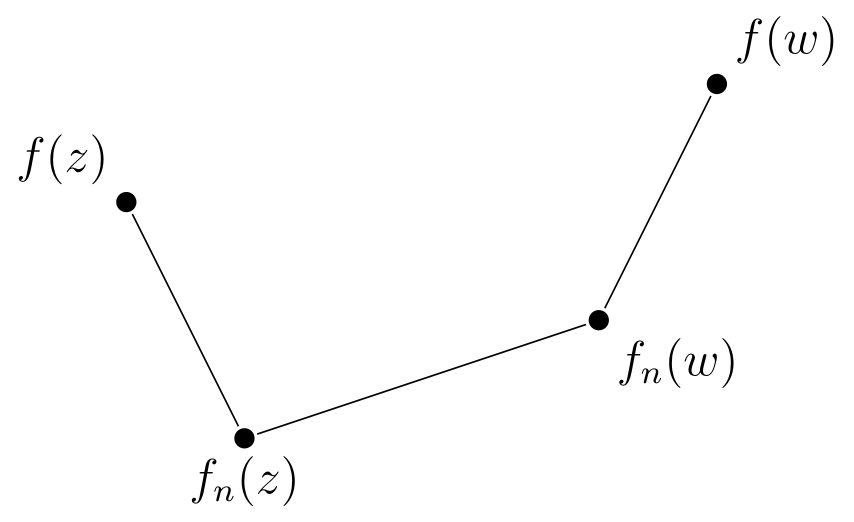
Show that if is a sequence of continuous functions that converge uniformly to on an open set , then is continuous on . You have to show that for any and any , there is a such that Hint: Fix . Choose big enough so that for all . Then use the continuity of and the triangle inequality (see the image below).
After that we talked about the idea that if a function is defined by a power series in a open disk, then you can often analytically continue the function by constructing a new power centered at a different point inside the open disk. In this way you can extend the function past its original disk of convergence. This has one immediate consequence. If a holomorphic function on an open connected domain has for all at one point , then everywhere in .
Theorem (Classification of Zeros) If is a holomorphic function in an open connected domain and for some , then either
everywhere on or
The Taylor series for centered at has a first nonzero term . In that case where is holomorphic in an open disk around and . Then we say that is a zero of order .
Find the orders for the following zeros:
for .
for .
Theorem (Zeros are Isolated) If is a non-constant analytic function in an open connected domain , then the zeros of are isolated which means that for every zero , there is an open disk around that does not contains any other zeros of .
Proof. By the classification of zeros theorem, for some where is holomorphic and . Then by continuity in an open disk around , except at .
Identity Principle. If is holomorphic on an open connected domain and has a sequence of distinct zeros that converge to a point , then everywhere on .
Why doesn’t the identity principle apply to the function which has infinitely many zeros in the open disk of radius one around 1?
This theorem is called the identity principle because it implies that if two holomorphic functions are the same on a compact (closed and bounded) infinite set inside , then they must the same on all of .
If is an open set, , and is holomorphic, then we say that is an isolated singularity of . There are three types of isolated singularities.
Here are examples of the three types of singularity.
at .
at .
at .
| Day | Section | Topic |
|---|---|---|
| Mon, Nov 4 | 9.1 | Classification of singularities |
| Wed, Nov 6 | 9.3 | The argument principle and Rouche’s theorem |
| Fri, Nov 8 | 8.3 | Laurent series |
Classification of Singularities. If has an isolated singularity at , then
is a removable singularity if and only if there is a holomorphic function on an open disk around such that everywhere, except (technically) on the disk.
is a pole if and only if there is a holomorphic
and positive integer
such that
for all
in an open disk around
and
.
We call
the order of the pole at
Prove that if , then is holomorphic at .
What can you say about the power series for centered at ?
If , then the function has a removable singularity at . What can you say about the power series for centered at ?
With this classification, we can prove a really cool theorem:
Argument Principle. Suppose that is holomorphic on an open simply connected domain , except for isolated poles. If is a piecewise smooth, positively oriented, simple closed path in and does not pass through any zeros or poles of , then the winding number of the path around the origin is
If has a zero at of order , then where is holomorphic, and Similarly, if has a pole at of order , then where is holomorphic, , and
If is the only zero or pole of inside , explain why this proves that the winding number of around is either or (depending on whether is a zero or a pole).
What if has several zeros and/or poles inside ?
The main application of the argument principle is not to find the winding number. It is actually to use the winding number to confirm the existence of zeros or poles.
Rouche’s Theorem. Suppose that are holomorphic on an open, simply connected domain , and is a positively oriented, simple, closed, piecewise smooth path in . If for all in the range of , then and have the same number of zeros inside (counting multiplicity).
Proof. The inequality condition is the same as the one for the dog on a leash theorem. Therefore and have the same winding numbers around the origin and then by the argument principle they must have the same number of zeros (they can’t have poles because they are holomorphic on ).
Open Mapping Principle. If is a non-constant holomorphic function on an open set , then is an open set.
Proof. We have to show that for every is an interior point of . In other words, there is an open disk around that is completely contained inside . By definition, there is a such that , and is a zero of the function . We just have to show that has a zero for all sufficiently close to .
Since zeros are isolated, we can choose a circle around in that doesn’t have any zeros on its boundary. Let be a positively oriented parametrization of that circle. Let be the distance from the closest point on to . If , then Rouche’s theorem guarantees that has a zero inside and therefore .
We ran out of time last class before we could write down this next corollary of the open mapping principle.
Maximum Modulus Principle. If is a non-constant holomorphic function on an open set , then cannot have a local maximum in . If in addition, is bounded and is continuous on the closure of , then the maximum of occurs on the boundary of .
Proof. Suppose that is a local maximum, that is, for all in a small disk around . This is a contradiction because is an open set, so it contains an open disk around .
A Laurent series centered at is a series of the form where the coefficients are complex numbers and is a complex variable. We say that a function has a Laurent series in a domain if there is a Laurent series that converges absolutely to for all . The sum of the terms of a Laurent series with negative powers is called the principal part and the sum of terms with nonnegative powers is the analytic part of a Laurent series.
We calculated Laurent series for the following functions in class.
.
.
We talked about how you can tell from the Laurent series above that 0 is an order 5 pole for the first example and an essential singularity in the second.
A function might have different Laurent series with the same center (unlike power series which are unique). Each Laurent series will converge in a different region. It is not hard to show that the region of convergence for a Laurent series is always an annulus, but we didn’t prove that in class.
Theorem. If has a Laurent series in an open annulus, then for any simple, closed, piecewise sooth curve in the annulus that winds around .
We proved this by using Cauchy’s theorem and Cauchy’s integral formulas to evaluate for every , and we saw that the only integral that wasn’t zero was when . The coefficient is called the residue of at .
| Day | Section | Topic |
|---|---|---|
| Mon, Nov 11 | 9.2 | Residues |
| Wed, Nov 13 | Review | |
| Fri, Nov 15 | Midterm 2 |
Residue Theorem. If is holomorphic in an open simply connected domain , except at some isolated singularities, and is a positively oriented, simple, closed, piecewise smooth path in that avoids the singularities of , then there are only finitely many singularities inside and where is the residue of at .
We talked about why this theorem is true. Then we looked at some examples.
.
Evaluate .
We got bogged down with the second example because we were trying to derive the formula for a residue every time from scratch.
Since we got held up last time with some tedious residue computations, I introduced the following formula today.
Theorem (Residue Formula). If has a pole at with order no more than , then
Proof. This follows from the fact that has a removable singularity at . So we could (in theory) find a power series for . Then the residue corresponds the -th order coefficient of the power series.
We applied the formula to the following examples:
Find the orders and residues of each pole of .
Evaluate .
We also did some review problems to prepare for the midterm including:
Use Rouche’s theorem to determine how many zeros has in the annulus with .
| Day | Section | Topic |
|---|---|---|
| Mon, Nov 18 | Contour integrals | |
| Wed, Nov 20 | 6.1 | Harmonic functions |
| Fri, Nov 22 | Vector fields & holomorphic functions |
Today we talked about applications of residues to real integrals. We started with the following result.
Theorem (Integrals of Rational Functions on the Real Line). If and are polynomials such that has no real zeros and the degree of is at least two greater than , then is times the sum of the residues of at all zeros of in the upper half plane.
After we sketched a proof, we applied this theorem to solve:
Another common type of problem that we can often solve using residues is or where is rational function that is continuous on the real axis. To evaluate these integrals, we can apply the Residue Theorem to either the real or imaginary part of . It helps to know the following inequality.
Jordan’s Lemma. Let
,
with
.
So
parametrizes the upper half of a circle of radius
around the origin. Then
Unfortunately the ML-inequality is not strong enough to prove this theorem. So we need to dig a little deeper into the integral.
Step 1. Show that if , then .
Step 2. Show that
Step 3. Show that
for all
.
Therefore
We started with this real integral
To convert integrals of functions involving sine & cosine from 0 to 2π, you can use the following substitutions, all based on letting and integrating over the unit circle:
After that, we introduced harmonic functions which are functions with continuous partial derivatives such that
Show that is harmonic.
Construct a real-valued function such that satisfies the Cauchy-Riemann equations.
Theorem (Harmonic Conjugates). If is harmonic on a simply connected open domain , then there exists a harmonic function such that is holomorphic. The function is called a harmonic conjugate of . The converse is true as well, if is holomorphic, then both the real and imaginary parts of are harmonic functions.
A corollary of the previous theorem and the open mapping principle is this:
Maximum Modulus Principle for Harmonic Functions. A harmonic function on a open domain cannot have a local max or local min in .
For a domain , we call a function a vector field on . If then the divergence and curl of are defined by
Green’s Theorem (both versions). If is a vector field in an open simply connected domain in that includes a simple, closed, piecewise smooth curve and let be the inside of . Then
where is the normal vector to at each point.
The div and curl versions of Green’s theorem explain the intuition that curl measures the net rotation of a flow (positive is counterclockwise, negative is clockwise), while divergence measures the net flux for the flow (inward is negative, outward is positive). When a vector field has everywhere, we say it is irrotational. When everywhere, we say that it is incompressible.
If is an open simply connected domain in , then any function can be thought of as a vector field. Furthermore, if is holomorphic on , then we know by Cauchy’s theorem that But keep in mind that That’s because complex multiplication is not the same as the dot-product on .
Recall that if and , then Therefore, if we let , then Since this is true on every small simple closed curve in , it follows that the vector field has everywhere.
The vector field is known as the Polya field of a holomorphic function . It turns out that the Polya field also has everywhere. To prove that, follow these exercises.
If , show that .
If is the normal vector for a path , then .
Show that .
From these you can conclude that:
So the Polya field of a holomorphic function is always both incompressible and irrotational. We ended with one more exercise that we didn’t have time to finish.
| Day | Section | Topic |
|---|---|---|
| Mon, Nov 25 | The heat equation | |
| Wed, Nov 27 | Thanksgiving break, no class | |
| Fri, Nov 29 | Thanksgiving break, no class |
We began with this exercise that we didn’t have time to finish last time.
Since is holomorphic, its Polya field is both irrotational and incompressible. We talked about why it makes sense that the gradient of a harmonic function would have those two properties, in light of the maximum modulus principle for harmonic functions.
Recall that a vector field on is conservative if there is a potential function such that is the gradient of . The Polya fields of a holomorphic function are all conservative. There are lots of applications of conservative vector fields. There are lots of examples of conservative vector fields in nature.
| Application | Potential Function | Tangent Curves | Normal Curves |
|---|---|---|---|
| Fluid flow | Pressure or elevation | Streamlines | Equipotential curves |
| Heat flow | Temperature | Lines of heat flux | Isotherms |
| Electrostatic force | Electric potential | Field lines | Equipotential curves |
Then we looked at the 2-dimensional heat equation:
This is a partial differential equation for modeling how the temperature at a point on a 2-dimensional object (like a thin metal plate) changes with respect to time . The solution would be a function that would tell us the temperature at any location and time. To understand where this equation comes from, consider the following:
The net flow of heat into a disk with boundary is equal to where is the (outward) normal vector and is the gradient of the temperature function (at a fixed time).
Note that the gradient points in the direction of greatest increase in temperature. If that is outwards (like in the image above), then it is hotter outside the disk , so heat tends to flow inwards (opposite the gradient vectors).
When the temperature reaches equilibrium, it stops changing so the left side of the heat equation () becomes zero. When that happens, is a harmonic function. We’ve talked about functions that are harmonic on the entire complex plane. But an important problem is to find functions that are harmonic on a domain that satisfy a boundary condition. This is called the Dirichlet problem.
The Dirichlet Problem. Let be a simply connected open domain with boundary Given a continuous real valued function defined on the boundary , find a continuous function on such that is harmonic in and on
| Day | Section | Topic |
|---|---|---|
| Mon, Dec 2 | The Dirichlet problem | |
| Wed, Dec 4 | Fourier transform | |
| Fri, Dec 6 | The heat equation | |
| Mon, Dec 9 | Recap & review |
We looked at one solution to the Dirichlet problem on the upper-half plane:
An important fact about harmonic functions and their conjugates is the following:
Theorem. If is a harmonic function and is its harmonic conjugate, then the level curves of are orthogonal to the level curves of .
Theorem. A harmonic function that is defined on one domain can be turned into a harmonic function on another domain if you can find an invertible holomorphic function . In that case, is a harmonic function on .
Prove this. Hint: there is a holomorphic function such that .
The Cayley transform is the Möbius transform which maps the upper half-plane into the unit disk. If , then what do the level curves of look like? Hint: recall that Möbius transforms send lines and circles to lines and circles.
Today we talked about the Fourier transform of a real function which is defined to be:
In class we used a contour integral to find the Fourier transform of
We also calculated the Fourier transform of the Gaussian . Before calculating that, we needed to know that . Here is a video that explains this.
Then we used a rectangular contour to show that .
Show that .
Use the contour below to show that in the limit as , so
We finished by talking about some of the properties of the Fourier transform.
Show that is linear, i.e.,
Prove the translation property: If , then
Prove the derivative property: Hint: Use integration by parts and use the fact that since must have a finite integral.
Today we used the Fourier transform to solve the 1-dimensional heat equation: with initial condition . The goal is to find an equation that can predict the temperature at any location and time on a thin rod.
We started by defining the convolution of two functions as
Convolutions play very nicely with the Fourier transform.
We need one more property of the Fourier transform before solving the heat equation.
Then we used these steps to solve the heat equation. Before we did that, we briefly talked about why the 1-dimensional heat equation makes sense.
Step 1. Apply the Fourier transform in the variable to both sides of the heat equation:
Step 2. Observe (without proof) that you can swap the integral and the partial derivative on the left side. And on the right side you can apply the derivative rule for Fourier transforms to get where is the Fourier transform of .
Step 3. Solve the ordinary differential equation
for
.
Step 4. Show that the inverse Fourier transform of is Hint: Apply the scaling and linearity properties to which we calculated last time.
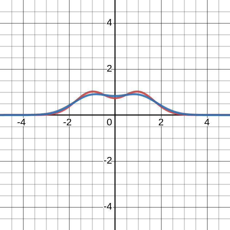
Step 5. Conclude that the solution of the heat equation is the convolution
In some cases you can calculate the value of this convolution by hand, but usually it is easier to use a computer to calculate it numerically. Here is a graph of an example solution of the heat equation on Desmos (click on the image below):
We went over some of the questions from the final exam. In particular, we talked about how to find the Fourier transform of a function that is only non-zero in a finite interval like the one in the exam. We did this example:
We also looked at what the solution of the heat equation would look like with this function as the initial condition. Surprisingly we don’t really need to know the Fourier transform of the initial condition since it goes away in the solution when we apply the inverse Fourier transform to get our final convolution equation for the solution.
We also talked about how to find a Laurent series.