Quick Links: Syllabus
| Week | Mon | Tue | Wed | Thu | Fri |
|---|---|---|---|---|---|
| 1 | Day 1 | Day 2 | Day 3 | Day 4 | |
| 2 | Day 5 | Day 6 | Day 7 | Day 8 | |
| 3 | Day 9 | Day 10 | Day 11 | Day 12 | Day 13 |
| 4 | Day 14 | Day 15 | Day 16 | Day 17 | Day 18 |
| 2 | Day 19 | Day 20 |
Today we introduced voting methods. See these slides for details.
We also did these two workshops in class.
Workshop: Plurality & Instant Run-Off Voting
Workshop: Borda Count
Today we talked about fairness criteria that voting methods should have.
We also did this workshop in class.
In addition to the slides & workshop, we also talked about (and proved) the Median Voter Theorem. We finished by talking about recent advocacy to promote ranked choice voting (another name for IRV) and STAR voting (which will not be on the test).
It is something to pay attention to in the future, because there will always be a push for better voting methods than plurality voting.
Today we talked about weighted voting systems. We did this workshop:
Before the workshop, we started with this example. Suppose a school is run by a committee with the principal who has 3 votes, the vice principal who has 2 votes, and three teachers who each have 1 votes. A motion requires 5 votes to pass.
We can use the shorthand notation [5: 3, 2, 1, 1, 1] to represent this weighted voting system. The first number is the vote threshold needed to pass a motion, and the other numbers are the weights which are the number of votes controlled by each voter. Often the voters in a weighted voting system are called players.
A winning coalition is a subset of the players who have enough votes to pass a motion. A player is critical in a winning coalition if the coalition would not have enough votes without that player.
List the winning coalitions in the weighted voting system above.
Circle the critical players in each winning coalition.
The Banzhaf power index is a way to measure how much power each player in a weighted voting system has.
To find the Banzhaf power for each player,
John Banzhaf was a lawyer in the 1960s who discovered the power index when he was investigating a case involving Nassua County, NY. The districts in Nassau county had a weighted voting system where the weights were:
To reach the threshold of 16 votes to pass a motion, it required at least two of the bigger districts. But it never mattered what the three smaller districts did. So the three smaller districts had no power in the elections.
A player with no power is called a dummy. A player with enough power to pass a motion all by themselves is called a dictator. Sometimes a player can block any motion by themselves. Then we say they have veto power.
Banzhaf power can illustrate some surprising things about weighted voting systems. For example, the weights might be very different from the real amount of power each player has.
Sometimes you can calculate the Banzhaf power indices without having any numbers for the weights and threshold. We did the following example.
If you want to play with more weighted voting examples, Professor Koether made a Banzhaf power calculator which you can try.
Today we talked about the spherical Earth theory. Actually, we talked about solving proportion equations, but most of the examples we did were related to the fact that the Earth is a sphere. We also talked about the evidence the ancient Greeks used to deduce that the Earth is a sphere.
After that, we talked about using the same ideas to find Latitude & Longitude.
We finished by talking about a useful technique to solve word problems involving unit conversions called factor-label method, also known as dimensional analysis. Here is a video explaining the technique (I didn’t make the video, but it is a pretty good explanation.
We did this example in class:
Then we finished with this workshop:
Today we talked about orders of magnitude. For any number, its order of magnitude is the exponent of the nearest power of 10. For example, 783 is closest to 1,000 which is , so the order of magnitude of 783 is 3. We also briefly reviewed scientific notation and the metric system. We did this workshop.
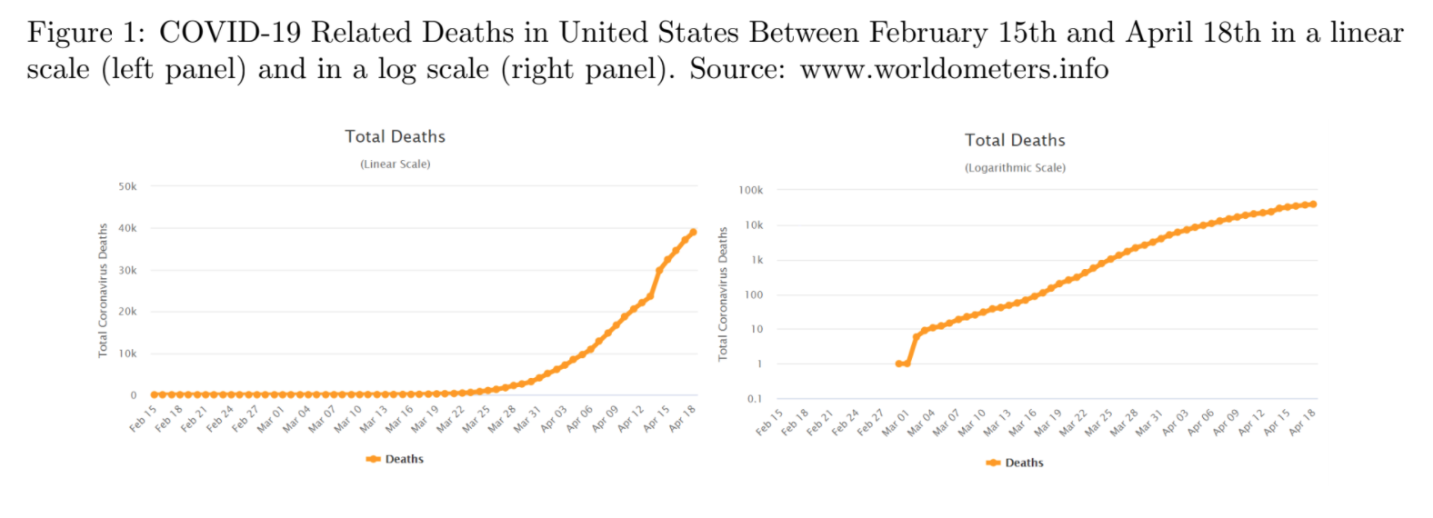
After that, we talked about logarithmic scales which are number lines where the numbers are spaced so that each step represents multiplication/division instead of addition/subtraction. We did this workshop
We also looked at examples where log-scales are used to present data. Sometimes these examples can be misleading. But sometimes a log-scale is the best way to represent the data.
Using log-scales to present data has advantages:
It spreads out small numbers so you can see them.
It lets you use one graph to represent numbers that are spread over many orders of magnitude.
The disadvantages are:
It bunches up the big numbers, so it can make big differences seem small.
They are more confusing because not everyone is familiar with log-scales.
We started by talking briefly about how the halfway point between two numbers on a logarithmic scale is not what you would expect. For example, the halfway point between 1 and 100 is 10, not 50. On a logarithmic scale, the halfway point between any two numbers and is the geometric mean which is:
The regular average where you add two numbers and then divide by 2 is called the arithmetic mean.
Fact. The arithmetic mean of two different positive numbers is always bigger than the geometric mean.
After we talked about arithmetic & geometric means, we introduced growth factors. When any quantity increases (or decreases), the growth factor is defined to be
Growth factors will be smaller than one if the quantity is decreasing.
When we work with growth factors that are close to one, we usually talk about percent change.
Percent changes are confusing because you can’t add and subtract percent changes. But you can multiply growth factors.
We did these two workshops.
After the break we talked about arithmetic and geometric sequences. An arithmetic sequence is a list of numbers that change by adding or subtracting a constant step size. A geometric sequence is a list of numbers that change by multiplying or dividing a constant factor, called the common ratio. Linear growth (or decrease) is when an arithmetic sequence is growing (or decreasing). Exponential growth (or decay) is when a geometric sequence is growing or decreasing.
We finished by watching this video about exponential growth and the rule of 70.
We started with a workshop.
Then we talked about logarithms. We talked about how (base-10) logarithms are pretty much the same thing as orders of magnitude. They tell you the exact location of a number on a logarithmic scale where each order of magnitude is one step.
Logarithms were discovered/invented by John Napier in the early 1600’s to help make arithmetic easier. Here is some of the history.
1614 John Napier published the book A Description of the Wonderful Rule of Logarithms.
1617 Henry Briggs published the first base-10 logarithm tables.
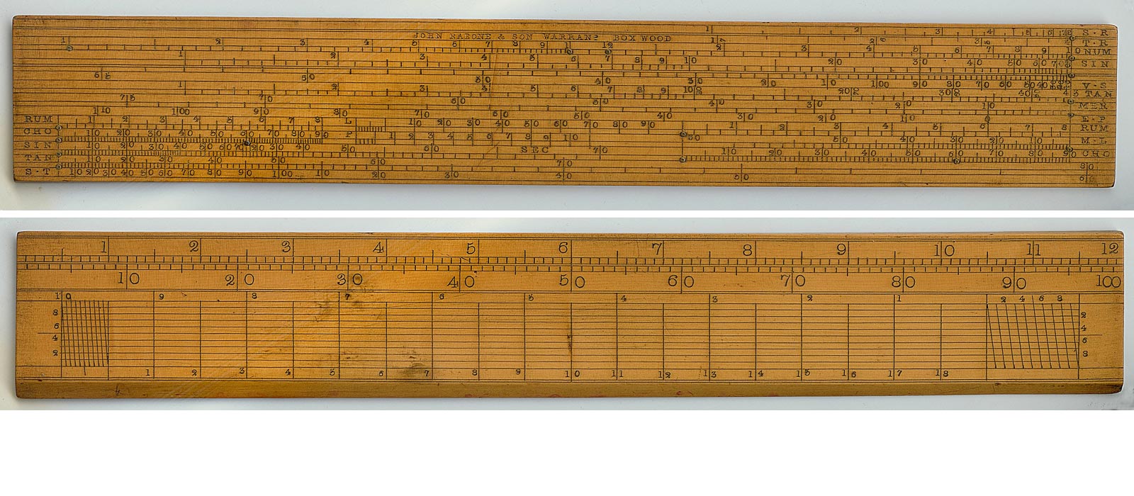
1624 Edmund Wingate published The Use of Rules of Proportion. A rule of proportion is a wooden ruler with numbers marked on a logarithmic scale. Wingate got the idea from Edmund Gunter and these rulers were sometimes called Gunter sticks.
Early 1630’s William Oughtred put two wooden rules of proportion together the make the first slide rule.
The reason that logarithms caught on so quickly is that they really did make people’s lives a lot easier.
Today we talked about the apportionment problem.
We also did this workshop
We also did an example where a Mom has 50 pieces of candy to give out to her 5 kids based on the number of minutes they spent doing chores.
| Alvin | Betty | Calvin | Daisy | Edwin | Total |
| 150 | 78 | 173 | 204 | 295 | 900 |
What is the standard divisor? What are its units?
What is the standard quota for each kid?
What is the apportionment using Hamilton’s method.
We finished by using a spreadsheet to find the apportionment of candy above using Jefferson’s method. We also used Jefferson’s method to find the final apportionment of Congress after George Washington vetoed the Apportionment Act of 1792.
Today we talked about advantages and disadvantages of the various apportionment methods. We also introduce the Huntington-Hill Method which is the one that the United States has used since 1941.
We did two workshops, the first involved using spreadsheets to implement divisor methods. You need to download the data file to do problem 2.
The other was a quick example of using a logarithmic scale to implement the Huntington-Hill method.
Today we introduced graph theory. We started by verifying Euler’s formula which says that any graph on a piece of paper with vertices, edges, and faces or regions (including the one exterior face which is not enclosed by edges), the following formula is always true:
A graph is a set of points called vertices and a set of lines connecting two vertices called edges (the edges don’t have to be straight). A graph that you can draw on a piece of paper so that no edges cross (except at vertices) is called a planar graph.
According to legend, the subject of graph theory was discovered/invented in 1735 when Leonhard Euler heard about the Seven Bridges of Königsberg puzzle. At the time, Königsberg was a city in Prussia with seven bridges. The puzzle asks whether it is possible to walk around the city crossing every bridge exactly once. Assume that you can only cross the river by walking across on of the bridges.
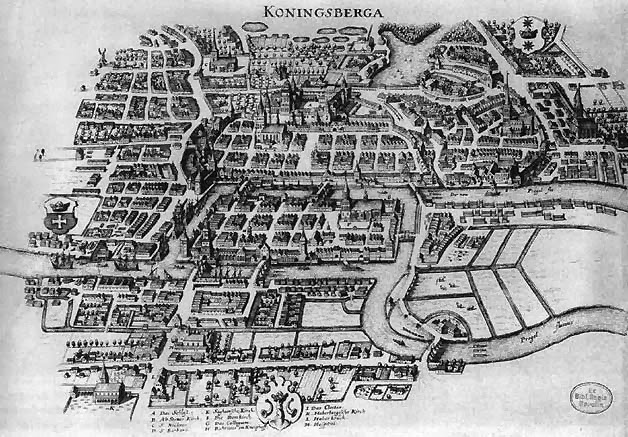
Euler solved the problem by abstracting away the irrelevant details and focusing on the underlying graph structure. A graph has an Euler path if there is a path that starts and ends at different vertices and crossed every edge exactly once. A graph has an Euler circuit if there is a path that starts and ends in the same place and crosses every edge exactly once.

Euler figured out that the only thing that matters (as long as the graph is connected) is the degrees of the vertices in the graph. The degree of a vertex is the number of edges that touch it.
Theorem. A connected graph has an Euler path if and only if it has exactly two vertices with an odd degree. A connected graph has an Euler circuit if and only if all of the degrees are even.
We didn’t prove this theorem, but we did give an intuitive explanation for why it is true. Cole also had an interesting idea that maybe you have to have an even number of edges to have an Euler path, but we ended up finding some counter examples for that conjecture.
We also proved this handy theorem:
The Handshake Theorem. In any graph, the sum of the degrees of all the vertices is twice the number of edges.
Then we did this workshop.
We also talked about Fluery’s algorithm, which is a way to find an Euler path (or circuit) in a graph.
Fluery’s algorithm. For a graph that has an Euler circuit (or path):
Pick a start vertex (must have odd degree if you are looking for a path).
Move along the graph from vertex to vertex, removing the edges you cross as you go. When you have a choice, never pick an edge that would make it impossible to reach some un-visited edges.
Continue until you are done.
It is not obvious, but this algorithm always works as long as a graph is connected and has only even degree vertices (or just two odd degree vertices).
Today we talked about trees. A tree is a graph that is connected and has no cycles. A path is a sequence of adjacent edges with no repeats. A cycle is a path of length more than 1 that never repeats an edges and starts and ends at the same vertex. We proved these theorems about trees, the most important of which is this first one (which includes several of the other theorems).
Tree Classification Theorem. For connected graphs, the following properties are equivalent. If a connected graph has one of these properties, then it has all of them.
The first part of the proof is to show that properties 1 and 2 are equivalent. We called this Tree Theorem 1. Here is why it is true. If there were two paths, then eventually they would split and then rejoin. The edges between where the paths split and rejoin would form a cycle, which is impossible. Conversely if there were a cycle, then there would be more than one path connecting any two vertices in the cycle (one going clockwise, the other counterclockwise).
To prove that property 3 is equivalent to the other two properties in the Tree Classification Theorem takes a little more work. We needed some helper theorems. The first theorem is about leaves which are vertices with degree one in a tree.
Theorem. Every tree with more than 1 vertex must have some leaves.
To prove this theorem, start from any vertex and make a path. Keep extending the path as long as you can, until you can’t go any farther. There are only two reasons you can’t go farther. Either you are at a dead end (which means you have found a degree one vertex), or you have already visited all the edges that touch the current vertex. But then the path has hit the vertex at least twice, and contains a cycle, which is impossible in a tree.
Theorem. For any tree, the number of vertices is always one more than the number of edges . In other words,
The key to proving this theorem is to use a technique called pruning. Since every tree must have some leaves (i.e., degree 1 vertices), you can remove a degree 1 vertex and the edge that touches it from the tree. After you do this, you will still have no cycles, and your graph will still be connected because any other two vertices will have a path connecting them. Therefore the pruned graph is still a tree, and so it still has more leaves you can prune. Each time you prune a vertex, you reduce the number of edges and vertices both by one, until you get down to a single vertex and no edges. At each step is the same, and at the end, , so in the original tree.
The last helper theorem we needed was about spanning trees. A spanning tree is a subgraph of a graph that is a tree and includes all of the vertices and some of the edges from the original graph.
Theorem. Every connected graph has a spanning tree.
This is true because if you start with a connected graph that has one or more cycles and remove one of the edges from a cycle, the new graph you get is still connected. So you can repeat the process until there are no more cycles left. When you are done, you have a connected subgraph with no cycles, i.e., a spanning tree.
With this last result, we were able to prove the final part of the Tree Classification Theorem: If a connected graph has exactly vertices, then it must be a tree. This is because a connected graph must have a spanning tree. The spanning tree has vertices. If the original graph also has vertices. Since both the original graph and the spanning tree have the same number of vertices, we conclude that they have the same number of edges, which means that the spanning tree is the original graph. So the original graph is a tree.
After developing all of this theory about trees, we introduced minimal spanning trees. In a connected graph where some edges are more expensive to include than others, the minimal spanning tree is the spanning tree that would be the least expensive to build. There is a simple algorithm to find the minimum spanning tree.
Kruskal’s Algorithm. To find the minimal spanning tree in a connected graph, follow these steps.
Add the cheapest edge.
Add the second cheapest edge (it doesn’t have to be next to the first edge).
Keep adding the cheapest edge available, as long as it doesn’t make a cycle. Stop when you have a tree.
We finished with this workshop.
Today we introduced Markov chains. We started with this example, which is from the book Introduction to Finite Mathematics by Kemeny, Snell, & Thompson.
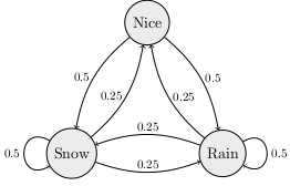
The Land of Oz is blessed by many things, but not by good weather. They never have two nice days in a row. If they have a nice day, they are just as likely to have snow as rain the next day. If they have snow or rain, they have an even chance of having the same the next day. If there is change from snow or rain, only half of the time is this a change to a nice day.
A Markov chain is a mathematical model with states and transition probabilities which only depend on the state you are currently in. The example above has three states: nice weather, rain, and snow. A Markov chain can be represented using a weighted directed graph. A directed graph is a graph where the edges have a direction (indicated by an arrow). A weighted graph is one where each edge has a number. In a Markov chain graph, the weights on the edges are the probabilities that you take that edge. Here is the graph for the weather in the Land of Oz.
Here is another example of a Markov chain.
A professor tries not to be late too often. On days when he is late, he is 90% sure to arrive on time the next day. When he is on time, there is a 30% chance he will be late the next day. How often is this professor late in the long run?
Draw and label a graph to represent this Markov chain.
If the professor is on time today, what is the probability that he will be on time the day after tomorrow?
There is another approach to Markov chains that makes it much easier to answer questions like the last one. For a Markov chain, the transition matrix is a rectangular array of numbers where the rows represent the possible current state, the columns represent the possible states in the next round. The number in row column of the matrix is the probability that you will end up in state if you started in state . For example, the transition matrix for the professor is:
| Late | On-Time | |
| Late | 0.1 | 0.9 |
| On-Time | 0.3 | 0.7 |
We usually don’t bother writing the names of the states (as long as we can remember the order). Then we just write the transition matrix this way:
You can model what we know about the current state using a probability vector which is a matrix with only one row and a probability for each possible state. The entries in a probability vector must add up to one. For example, here are two different probability vectors: The first would represent being 100% sure that the professor is on-time. The second shows a 40% chance that the professor is late and a 60% chance that he is on-time.
Fact. If is the transition matrix for a Markov chain and is a probability vector indicated what we know about the current state, then is the probability vector for the next state.
In order to calculate times , you need to know how to multiply matrices. Here are some videos that explain how to multiply matrices: (https://youtu.be/kT4Mp9EdVqs and https://youtu.be/OMA2Mwo0aZg).
You can also raise a matrix to a power. For example, , just means times , and is . For transition matrices, represents how the Markov chain will change in 2 rounds and represents how the Markov chain will change in 3 rounds. Higher powers just represent more transitions.
We used the Desmos Matrix Calculator to calculate for the late professor Markov chain, and we found that no matter whether the professor was late or on-time the first day, there is a roughly 25% chance he will be late 10 days later. We finished with this workshop.
Today we continued talking about Markov chains. We started by looking at the transitions matrices for both the tardy professor example and the weather in the Land of Oz example from last time. In both cases, when you raise the matrices to larger and larger powers, the results get closer and closer to a single matrix. When that happens, we say that the matrices converge.
What often tends to happen is that after a large number of transitions, we get a probability vector that doesn’t change. A probability vector such that is called a stationary distribution. It turns out that all Markov chains have a stationary distribution. If the powers of the transition matrix converge, then each row of the matrix that they converge to is a stationary distribution for the Markov chain.
You can tell a lot about a Markov chain by looking at the strongly connected components of its graph.
Definition. A directed graph is strongly connected if you can find a path from any start vertex to any other end vertex . A strongly connected component of a graph is a set of vertices such that (i) you can travel from any one vertex in the set to any other, and (ii) you cannot returns to the set if you leave it. Strongly connected components are also known as classes. Every vertex of the graph will always be contained in exactly one class. A class is final if there are no edges that leave the class.

In the directed graph above, there is one final class and two other non-final classes. States in a Markov chain that are not in a final class are called transitory. A state that you can enter but never leave is called absorbing. We looked at this example of a Markov chain with an absorbing state.
Suppose McDonald’s is having a Teenage Mutant Ninja Turtles special where each happy meal comes with a toy figure of one of the four ninja turtles (each equally likely). Suppose that a kid buys a happy meal every day to try to collect all four turtles.
Draw the graph for this Markov chain. Hint: The states can just be the number of different turtles the kid has collected so far.
What is the transition matrix for this Markov chain?
What is the probability of getting all four turtles if you buy 7 happy meals?
How many happy meals would it take for there to be at least a 90% probability of having all four turtles?
We finished with a second workshop about Markov chains.
Today we talked about probability theory. We started by defining probability models.
A probability model has two parts:
A set of possible outcomes called the sample space, and
A probability function which assigns a probability to each outcome in the sample space.
We talked about how everyone has a mental model of how flipping a coin works and how rolling a six-sided die works. Those are both examples of probability models. A probability model is equiprobable if every outcome is equally likely. Both the fair coin and six-sided dice models are equiprobable. A simple probability model that is not equiprobable would be if you flipped two fair coins and counted the number of heads.
We drew a probability histogram for this model, which is just a bar chart that shows the probability for each outcome. This is also called a probability distribution.
After the first distribution we talked about the basic rules of probability. First, we defined an event which is any subset of the sample space. We often use capital letters like A or E to represent events. We use the shorthand to mean: the probability that event E happens. In an equiprobable space there is a simple formula for the probability of an event: $$P(E) = .
The other rules we talked about are these:
Complementary Events For any event ,
Addition Rule For any two events and ,
Multiplication Rule for Independent Events If and are independent events, then
Two events are independent if the probability that happens does not change if happens. Here is an example:
We also did this example:
35% of voters in the US identify as independents and 23% of voters call themselves swing voters. 11% of voters are both.
What is the probability that a voter is independent or a swing voter?
What is the probability that a voter is neither indpendent nor a swing voter?
How can you tell that being an indpendent voter is not indepdent of being a swing voter?
We finished with this workshop:
Today we talked about weighted averages and expected value. We started by reviewing how to calculate a weighted average. A weighted average is the dot-product of a list of numbers with a list of weights. The weights should be fractions or decimals that add up to one.
Suppose that the final grade in one class is based on the following components:
|
Project |
Midterms |
Quizzes |
Final |
|
5% |
45% |
20% |
30% |
Calculate the final average for a student who got 100 on the project, 73 on the midterms, 89 on the quizzes, and 81 on the final.
11 nursing students just graduated. Four of the students graduated in 3 years, four took 4 years, two finished in 5 years, and one student took 6 years to graduate. Express the average number of years it took the students as a weighted average.
After we reviewed weighted averages, we talked about how there are two different kinds of averages that are important in probability theory.
Sample mean - This is the regular average when you look at the outcomes of a repeated random experiment.
Theoretical mean (also known as the expected value) this is the weighted average of the possible outcomes, using the probabilities as the weights.
One confusing thing is that you don’t expect to get the “expected value” if you only roll a die once. To understand what we mean when we call the theoretical mean the expected value, you need to know the Law of Large Numbers:
The Law of Large Numbers. If you repeat a random experiment, the sample means tends to get closer to the theoretical mean as the number of trials increases.
After the workshop, we introduced weighted tree diagrams, which are a tool to help keep the addition and multiplication rules in probability straight. We started with this example:
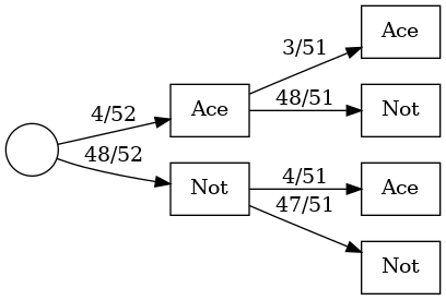
Weighted Tree Diagrams.
Notice that the multiplication rule we talked about last time requires events to be independent. A more general multiplication rule that does not assume events are indpendent is the following:
We finished with this exercise:
Today we talked about conditional probabilities .
Conditional Probability Formula. For any two events A and B, the conditional probability of A given B is
This comes directly from the multiplication rule we talked about last time. We started with the following example.
| Inoculated | Not Inoculated | Total | |
| Lived | 238 | 5136 | 5374 |
| Died | 6 | 844 | 850 |
| Total | 244 | 5980 | 6224 |
The probability that someone died if they were inoculated was only . The probability of dying for un-inoculated people was much higher, . Both of these are conditional probabilities of the form . What is the A and B for each?
Conditional probabilities can be surprisingly counter-intuitive.
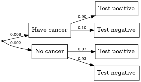
What percent of women test positive for breast cancer?
What is the probability that a woman actually has breast cancer given that they test positive?
After the workshop we briefly went over some questions about the midterm 2 review problems.
Today we introduced the normal distribution. Lots of things in nature have a probability distribution that is shaped like a bell. Here are some examples.
Another important example is when you flip a coin (fair or unfair) many times and count the number of heads. The total number of heads has a distribution called the binomial distribution that has a shape that looks more and more like a bell curve as the number of flips gets larger and larger.
In fact, one of the most important mathematical facts is that any time you add independent random numerical outcomes that come from a fixed probability distribution, the results tend to have a normal distribution as the number of observations increases. The normal distribution is a probability model that has a complicated formula, but it also has the following simple features.
Fact. A normal distribution is completely described by the two numbers and . The reason that normal distributions are so common in math & nature is the following theorem.
The Central Limit Theorem. The sum of a large number of independent observations from a probability distribution tends to have a normal distribution. The distribution of the sum gets more normal as increases.
We also talked about the 68-95-99.7 Rule:
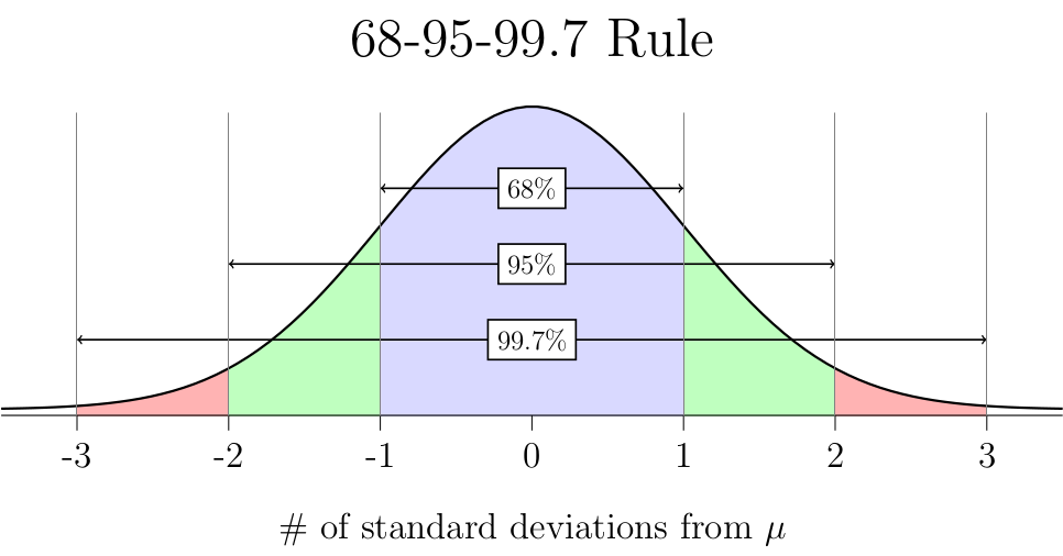
When working with normal distributions, it is common to refer to data in terms of how many standard deviations it is above or below the mean. This is called standardized data or z-values. The formula to calculate a z-value is:
We used z-values to answer the following question.
After we did the workshop, we talked about roulette again. If you bet on black, then you win with probability 18/38, but if you bet on a number like 7, then you only win 1/38 times. But since the payoff is bigger if you bet on a number, you still get the same theoretical average payoff ($0.947 for every dollar bet). But even though both bets have the same , they actually have very different probability distributions if you play 100 games.
How many games would you expect to win if you play 100 games and bet on black every time?
Is the probability histogram for the total number of wins approximately normal in this case?
How many games would you expect to win if you play 100 games and bet on 7 every time?
Is the probability histogram for the total number of wins approximately normal in this case?
It turns out that you are much more likely to beat the house if you bet 100 times on 7 than if you bet 100 times on black. We finished by talking about risk (which is measured by the standard deviation) can be weighed against the expected value of the reward to judge whether investments are worthwhile.
Today we talked about binary outcome models which are probability models where each trial has only two possible outcomes, and we assume that the trials are independent and the probability of a success is the same every try. In a binary outcome model with trials and a probability of a success on each, the total number of successes has:
Theoretical average , and
Standard deviation .
If is large enough, then the distribution of successes will be approximately normal. A nice rule of thumb for when is large enough is the following: if there are at least 10 possible outcomes above and below the theoretical outcome , then the distribution of the number of successes will be approximately normal. We looked at a couple of examples.
In roulette, if you play 100 games and bet on black, you have a probability of winning of each round. What is the theoretical average and standard deviation for the number of games won? Is it appropriate to use a normal distribution to model this situation?
In roulette, if you play 100 games and bet on 7, then you have a probability of winning of each round. What is the theoretical average and standard deviation for the number of games won? Is it appropriate to use a normal distribution to model this situation?
In the 1920s, the number’s racket was an illegal lottery run by the mob in big cities. Anyone could buy a numbers ticket for $1. You could pick any three digit number, including 000. At the end of the day, there was a drawing and anyone who picked the winning number would win $600.
Suppose someone bought 300 tickets per year, every year, for a whole decade. How many times would they win on average? Would the number of times they won be approximately normal? Why not?
It is estimate that some organized criminals sold as many as 150,000 tickets per week. How many of those tickets would be winners, on average? What is the standard deviation? Is a normal approximation appropriate here?
You can test someone to see if they are psychic using Zener cards. If someone is just guessing, they should only get about 20% of their guesses right. Assuming that someone is just guessing (doesn’t really have psychic powers) is called the null hypothesis. It would take some very strong evidence to convince me that the null hypothesis is wrong and someone really has psychic powers. Out of 25 trials, how many would you expect to be correct if they are just guessing? What is the standard deviation for the number of correct guesses?