| Day | Section | Topic |
|---|---|---|
| Mon, Aug 25 | 1.1 | Modeling with Differential Equations |
| Wed, Aug 27 | 1.2 | Separable Differential Equations |
| Fri, Aug 29 | 1.3 | Geometric and Quantitative Analysis |
We talked about some examples of differential equations.
We talked about dependent and independent variables, the order of a differential equation and how to tell if a function is a solution of a differential equation. We also talked about initial conditions.
Spring-Mass Model. The force of a mass at the end of a spring can be modeled by Hooke’s Law which says where is the displacement of the spring from its rest position.
The last question led to a discussion of linear versus non-linear differential equations. It’s usually much harder to solve non-linear equations! We will also study systems of differential equations, like the following.
Here is a graph showing these equations as a vector field (with constants ).
Logistic Growth. where is a proportionality constant and is the carrying capacity.
Today we talked about separable equations. We solved the following examples.
Solve .
Solve . (https://youtu.be/1_Q4kndQrtk)
Not every differential equation is separable. For example: is not separable.
Which of the following differential equations are separable? (https://youtu.be/6vUjGgI8Dso)
We finished with this example:
Newton’s Law of Cooling. The temperature of a small object changes at a rate proportional to the difference between the object’s temperature and its surroundings.
Mixing Problem. Salty water containing 0.02 kg of salt per liter is flowing into a mixing tank at a rate of 10 L/min. At the same time, water is draining from the tank at 10 L/min.
We didn’t get to this last example in class, but it is a good practice problem.
Today we talked about slope fields.
Here is a slope field grapher tool that I made a few years ago. You can also use Sage to plot slope fields. Here is an example from the book, with color added.
t, y = var('t, y')
f(t, y) = y^2/2 - t
plot_slope_field(f, (t, -1, 5), (y, -5, 10), headaxislength=3, headlength=3,
axes_labels=['$t$','$y(t)$'], color = "blue")Consider the logistic equation with harvesting. where is a number of rabbits that are harvested each year.
The logistic equation (with or without harvesting) is autonomous which means that the rate of change does not depend on time, just on . An equilibrium solution for an autonomous differential equation is a solution where for all .
| Day | Section | Topic |
|---|---|---|
| Mon, Sep 1 | Labor day - no class | |
| Wed, Sep 3 | 1.7 | Bifurcations |
| Fri, Sep 5 | 1.6 | Existence and Uniqueness of Solutions |
Last time we talked about equilibrium solutions of autonomous equations. An equilibrium for is stable (also known as a sink or attactor) if any solution with initial value close to converges to as . An equilibrium is unstable (also known as a source or repeller) if all solutions move away from as .
We talked about the phase line for an autonomous ODE.
Suppose that is a family of differential equations that depends on a parameter . A bifurcation point is a value of the parameter where the number of equilibrium solutions changes. A bifurcation diagram is a graph that shows how the phase lines change as the value of a parameter changes.
You can use Desmos to help with the previous problem. Using to represent , you can graph the region where is positive in blue and the region where is negative in red. Then it is easier to draw the phase lines in the bifurcation diagram.
Today we talked about two important theorems in differential equations.
Existence Theorem. Suppose that where is a continuous function in an open rectangle . For any inside the rectangle, there exists a solution defined on an open interval around such that .
This theorem guarantees that in most circumstances, we are guarantee to have solutions to differential equations. But there are things to watch out for. Solutions might blow up in finite time, so they might not be defined on the whole interval .
Uniqueness Theorem. Suppose that where both and its partial derivative are continuous in an open rectangle . Then for any , there exists a unique solution defined on an open interval around such that .
If the partial derivative is not continuous, then we might not get unique solutions. Here is an example.
One very nice consequence of the uniqueness theorem is this important concept:
No Crossing Rule. If and are both continuous, then solution curves for the differential equation cannot cross.
This illustrates that a formula for a solution to might not apply after we reach a point where is no longer continuous.
| Day | Section | Topic |
|---|---|---|
| Mon, Sep 8 | 1.4 | Analyzing Equations Numerically |
| Wed, Sep 10 | 1.4 | Analyzing Equations Numerically - con’d |
| Fri, Sep 12 | 1.5 | First-Order Linear Equations |
Many ODEs cannot be solved analytically. That means there is no formula you can write down using standard functions for the solution. This is true even when the existence and uniqueness theorems apply. So there might be a solution that doesn’t have a solution you can write down. But you can still approximate the solution using numerical techniques.
Today we introduced Euler’s method which is the simplest method to numerically approximate the solution of a first order differential equation. We used it to approximate the solution to
from numpy import *
import matplotlib.pyplot as plt

def EulersMethod(f,a,b,h,y0):
    '''
    Approximates the solution of y' = f(t, y) on the interval a < t < b with initial
    condition y(a) = y0 and step size h.
    Returns two lists, one of t-values and the other of y-values.
    '''
    t, y = a, y0
    ts, ys = [a], [y0]
    while t < b:
        y = y + f(t,y)*h
        t = t + h
        ts.append(t)
        ys.append(y)
    return ts, ys

f = lambda t,y: y**2 / 2 - t

# h = 1
ts, ys = EulersMethod(f, -1, 5, 1, 0)
plt.plot(ts,ys)
# h = 0.1
ts, ys = EulersMethod(f, -1, 5, 0.1, 0)
plt.plot(ts,ys)
# h = 0.01
ts, ys = EulersMethod(f, -1, 5, 0.01, 0)
plt.plot(ts,ys)
plt.show()
Here’s the output for this code and here is a version with the slope field added.
After demonstrating how to implement Euler’s method in code, we talked about some simpler questions that we can answer with pencil & paper.
Euler’s method is only an approximation, so there is a gap between the actual y-value at and the Euler’s method approximation. That gap is the error in Euler’s method. There are two sources of error.
As
gets smaller, the discretization error gets smaller, but the rounding
error gets worse.
A worst case upper bound for the error is:
where
,
,
and
is the smallest floating point number our computer can accurately
represent. Using the standard base-64 floating point numbers,
.
In practice, Euler’s method tends to get more accurate as
gets smaller until around
.
After that point the rounding error gets worse and there is no advantage
to shrinking
further.
Today I announced Project 1 which is due next Wednesday. I’ve been posting Python & Sage code examples, but if you would rather use Octave/Matlab, here are some Octave code examples.
Runge-Kutta methods are a family of methods to solve ODEs numerically. Euler’s method is a first order Runge-Kutta method, which means that the discretization error for Euler’s method is which means that the error is less than a constant times to the first power.
Better Runge-Kutta methods have higher order error bounds. For example, RK4 is a popular method with fourth order error . Another Runge-Kutta method is the midpoint method also known as RK2 which has second order error.
Midpoint Method (RK2). Algorithm to approximate the solution of the initial value problem on the interval with initial condition .
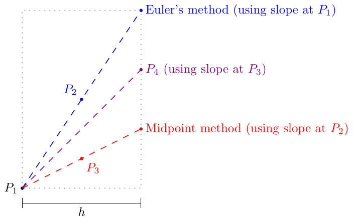
In RK2 the slope used to calculate the next point from a point is the slope at the midpoint between and the Euler’s method next step. In RK4, the slope used is a weighted average of the slopes at , , , and shown in the diagram above. Specifically, it is 1/6 of the slopes at and plus 1/3 of the slopes at and .
There are even higher order Runge-Kutta methods, but there is a trade-off between increasing the order and increasing complexity.
After we talked about Runge-Kutta methods, we introduced the integrating factors method for solving first order linear ODEs The key idea is that if is an antiderivative of , then is an integrating factor for the ODE. Since by the product rule, we can re-write the ODE as: Then just integrate both sides to find the solution.
Today we looked at more examples of linear first order ODEs.
Write down an IVP to model this situation using to represent the amount of salt in the tank.
Use integrating factors to solve the IVP. (https://youtu.be/b5QWC2DA5l4)
Sometimes it can be faster to use a guess-and-check method instead of integrating factors to solve linear ODEs. Here is an example. Consider the first order linear ODE: You might guess that there is a constant such that is a solution of this differential equation. This is true!
So is one particular solution for this ODE. To get all of the solutions, we need some theory:
A first order linear differential equation is homogeneous if it can be put into the form Any inhomogeneous equation has a general solution where
| Day | Section | Topic |
|---|---|---|
| Mon, Sep 15 | 2.1 | Modeling with Systems |
| Wed, Sep 17 | 2.2 | The Geometry of Systems |
| Fri, Sep 19 | 2.4 | Solving Systems Analytically |
Consider the inhomogeneous linear ODE:
If you know that waves can be modeled by equations of the form
,
then you might guess that the solution
might have this form. Then substituting into the equation, we get
By combining like terms, we get a system of equations
The solution is
,
which means that
is one solution to the ODE.
What is the corresponding homogeneous equation, and what is its solution?
What is the general solution to ?
Why is the method of integrating factors harder here?
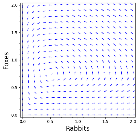
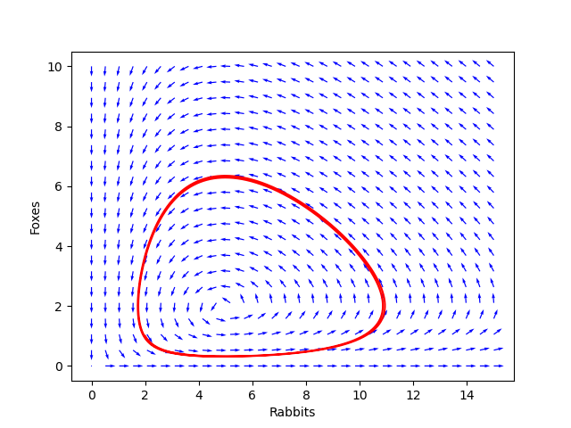
After that, we introduced systems of differential equations. We started with this simple model of a predator-prey system with rabbits and foxes :
A graph of the vector field defined by a system of two differential equations is called a phase plane. Solution curves are parametric functions and that follow the vector field in the phase plane.
According to Hooke’s law the force of a spring is or equivalently This is a homogeneous 2nd order linear differential equation.
We can convert a second order ODE to a first order system of equations by using an extra variable equal to the first derivative . Then , so we get the system:
Today we looked at more examples of systems of ODEs.
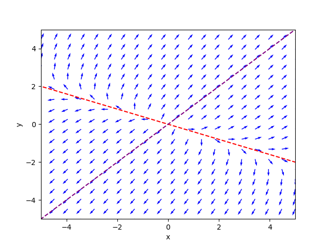
Suppose that we have two species that compete for resources and their populations and satisfy
Later in chapter 3 we will learn how to classify different types of equilibrium solutions on the phase plane using linear algebra. For now, here is a preview of some of the types of equilibria.
A simple model used to understand epidemics is the SIR-model, which stands for Susceptible-Infected-Recovered. The idea is that a disease will spread from people who are infected to people who are still susceptible. After infected people recover, they are usually immune to the disease, at least for a little while. In the system below, is the percent of the population that is still susceptible, is the percent that are currently infected, and is the percent of the population that are recovered. The constants and are the transmission rate and recovery rate, respectively.
Under what circumstances is the number of infected people increasing?
If we introduce a vaccine, what effect might that have on the model?
What if the disease is fatal for some people? How would you change the model to account for that? Hint: You could have a constant that represents the fatality rate, i.e., the proportion of the infected population that die each day.
If you divide by , you get the differential equation Solve this differential equation with initial condition and .
Here is a plot showing the solution superimposed on the direction field (for and only).
Today we talked about decoupled systems and partially coupled systems.
A system of equations is called decoupled since the -variable doesn’t depend on , and the -variable doesn’t depend on . You can solve the differential equations in a decouple system separately.
A system of equations is partially coupled. You can solve for first, and then substitute into the first equation to create a single variable differential equation for .
Solve the system
Solve the system with initial conditions and . (https://youtu.be/sJ3CuM-QmOk)
Here is a Desmos graph showing the solutions to the last problem as different parametric curves.
| Day | Section | Topic |
|---|---|---|
| Mon, Sep 22 | 2.3 | Numerical Techniques for Systems |
| Wed, Sep 24 | C1 | Complex Numbers and Differential Equations |
| Fri, Sep 26 | C2 | Solving System Analytically - con’d |
Today we introduced Euler’s method for systems of differential equations equations.
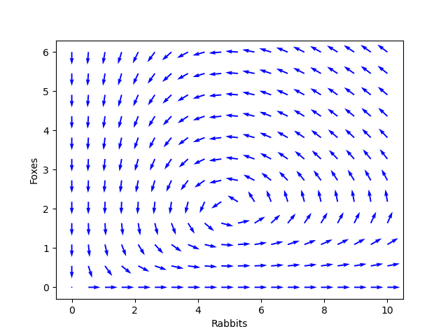
A more realistic model for the rabbits & foxes might be if the rabbits growth was constrained by a carrying capacity of 10 thousand rabbits (logistic growth), in the absence of foxes. How would this change the differential equation above?
Now use Euler’s method to investigate the long-run behavior of the rabbits & foxes with this new model. What changes?
Now talk about the equation for a pendulum:
Typically in introductory physics, you find an approximate solution of this equation by assuming that the angle stays small and so . But we can use Euler’s method instead to generate solutions numerically (Python).
Today we introduced complex numbers and talked about how they can arise in differential equations.
A complex number is an expression where are real numbers and has the property that .
The real-part of is and the imaginary part is .
The absolute value .
The complex conjugate of is .
Calculate .
Show that for any complex number .
Euler’s Formula.
A complex-valued function is a function where both and are real-valued functions. You can integrate and differentiate complex-valued functions by integrating/differentiating the real and imaginary parts.
Polar Form. Any complex number can be expressed as , where and is an angle called the argument of .

Convert and to polar form, then multiply them by applying the formula
Solve the differential equation .
Show that is a solution for the differential equation . Hint: The chain rule applies to complex-valued functions, so .
Today we talked about homogeneous second order linear differential equations with constant coefficients.
These equations are used to model simple harmonic oscillators such as a spring where the total force depends on a spring force and a friction or damping force :
General Solution of a 2nd Order Homogeneous Linear Differential Equation.
Theorem. If and are linearly independent solutions of then the general solution is
Using the language of linear algebra, we can describe the result above several ways:
We applied the theorem above to the following two examples:
Find the general solution to . (https://youtu.be/Pxc7VIgr5kc?t=241)
Find the general solution of . Hint: Use the quadratic formula.
| Day | Section | Topic |
|---|---|---|
| Mon, Sep 29 | Review | |
| Wed, Oct 1 | Midterm 1 | |
| Fri, Oct 3 | 3.1 | Linear Algebra in a Nutshell |
We talked about the midterm 1 review problems. We also looked at this example:
Today we talked about homogeneous linear systems of differential equations. These can be expressed using a matrix. For example, if , then the system of differential equations can be re-written as It turns out that the eigenvectors and eigenvalues of tell you a lot about the solutions of the system. We did these exercises in class.
Find the characteristic polynomial and eigenvalues of the matrix
Show that is an eigenvector for . What is its eigenvalue?
Find an eigenvector for corresponding to the eigenvalue by finding the null space of .
After those examples, we did a workshop.
We also talked about how to calculate the eigenvectors of a matrix
using a computer. In Python, the sympy library lets you
calculate the eigenvectors of a matrix exactly when possible. You can
also do this in Octave if you load the symbolic
package.
from sympy import *

A = Matrix([[3,5],[2,6]])
'''
The .eigenvects() method returns a list of tuples containing:
1. an eigenvalue,
2. its multiplicity (how many times it is a root), and
3. a list of corresponding eigenvectors.
'''
pretty_print(A.eigenvects())| Day | Section | Topic |
|---|---|---|
| Mon, Oct 6 | 3.2 | Planar Systems |
| Wed, Oct 8 | 3.2 | Planar Systems - con’d |
| Fri, Oct 10 | 3.3 | Phase Plane Analysis of Linear Systems |
Today we talked about how to solve a homogeneous linear system using the eigenvectors and eigenvalues of when the eigenvalues are all real with no repeats. We did the following examples:
Solutions of Homogeneous Linear Systems.
Fact. If is an eigenvector of with eigenvalue , then is a straight-line solution for the linear system .
Fact 2. The general solution of a planar system with distinct real eigenvalues and corresponding eigenvectors is
We used these facts to find the general solutions for the following systems.
We also talked about how to graph the solutions.
We finished with the following question:
Last time we talked about how to find general solutions for linear systems. Today we talked about how to find specific solutions that satisfy an initial condition. Before that, we answered this question:
Under what circumstances does have more than one equilibrium solution?
Any time that zero is an eigenvalue of (i.e., the null space of is non-trivial), all of the eigenvectors corresponding to zero (i.e., the vectors in the null space) will be equilibrium points. It helps to know following theorem:
Invertible Matrix Theorem. For an n-by-n matrix , the following are equivalent.
After that, we talked about the classification of equilibria for linear systems.
Types of Equilibria for Planar Systems with Real Eigenvalues.
Then we solved the following initial value problems.
Find the solution to that satisfies
Find the solution to that satisfies
We used row reduction to solve these initial value problems. Here’s a video with a similar exercise (https://youtu.be/Mnz-S-RvpDw) if you want a different take. Octave makes this kind of matrix computation very easy.
pkg load symbolic
A = sym([3 5; 2 6])

# The columns of V are the eigenvectors and the diagonal entries of D are the eigenvalues.
[V, D] = eig(A)

# The backslash operator A \ b solves the matrix equation Ax = b.
V \ [7;0]Today we talked about systems with complex eigenvalues. We started by looking at three different direction fields for the following three matrices:
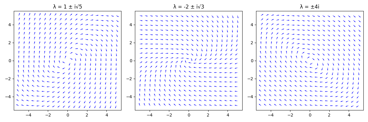
Types of Equilibria for Planar Systems with Complex Eigenvalues.
Suppose is a planar system with complex eigenvalues .
We talked about why this is true using Euler’s formula
It is still true that the general solution is but the coefficients are typically complex numbers and we only want real solutions. Next time we’ll discuss a better way to find the real-valued solutions.
| Day | Section | Topic |
|---|---|---|
| Mon, Oct 13 | Fall break - no class | |
| Wed, Oct 15 | 3.4 | Complex Eigenvalues |
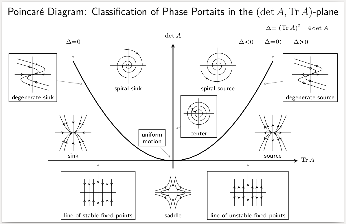
| Fri, Oct 17 | 3.7 | The Trace-Determinant Plane |
Last time we talked about planar systems with complex eigenvalues. We haven’t seen how to find nice solutions for those systems yet. Here is the key idea we need:
Solutions for Systems with Complex Eigenvalues.
Fact. If is a complex solution to a real linear system , then both the real and imaginary parts of are real solutions for the system.
Fact 2. If is a complex solution of a planar system where the real-part and the imaginary-part are linearly independent when , then the general solution is
Here’s how to use these facts to find the general real-valued solution:
Step 1. Find an eigenvector and its corresponding eigenvalue . Then is one complex solution for the system.
Step 2. Use Euler’s formula to convert
Step 3. Expand to find the real and imaginary parts.
We used this approach to find the general (real) solutions for the following planar systems.
Suppose a planar system has an eigenvector with corresponding eigenvalue . What is the general solution for the system?
Find a solution for the previous example with initial condition .
If you change the parameters of a system of differential equations, a bifurcation happens when the type or number of equilibria changes. For planar systems, that happens when , , or when .
Consider the 1-parameter family . For what values of do you get bifurcations?
Consider the harmonic oscillator .
Here are two more examples that we didn’t have time for in class.
Consider the 1-parameter family . For what values of do you get bifurcations? (https://youtu.be/F2ew7_dD5Zg)
Consider the 2-parameter family . Describe how the type of equilibrium depends on the parameters and .
| Day | Section | Topic |
|---|---|---|
| Mon, Oct 20 | 3.9 | The Matrix Exponential |
| Wed, Oct 22 | 3.8 | Linear Systems in Higher Dimensions |
| Fri, Oct 24 | 3.5 | Repeated Eigenvalues |
Today we talked about the matrix exponential and how it solves any homogeneous linear system!
The Matrix Exponential.
Definition. For any -by- matrix ,
Fact. is the solution of the system with initial condition .
To calculate a matrix exponential, start by diagonalizing the matrix, if possible.
Diagonalization Theorem.
If an -by- matrix has linearly independent eigenvectors with corresponding eigenvalues , then where
Furthermore, the matrix exponential for a diagonalizable matrix is:
To solve the last problem, it helps to know the following formula.
Inverse of a 2-by-2 Matrix.
Use the diagonalization of to solve the initial value problem
Calculate for and use it to find the general solution to . Hint: the eigenvalues of are with corresponding eigenvectors .
Since calculating a matrix exponential by hand is so tedious, we’ll usually use a computer.
Be careful computing symbolic matrix exponentials. It only works for very simple matrices.
Today we talked about homogeneous linear systems in 3-dimensions. We started with these examples.
Use the matrix exponential function to find the solution to the initial value problem
Use Desmos 3D to graph the solution above.
Find the straight-line solutions and the general solution for the system Hint: The matrix for this system has eigenpairs
Consider the system .
There is one other case of linear systems that we haven’t considered yet. What happens when there are repeated eigenvalues?
Linear Systems with Repeated Eigenvalues.
If is a 2-by-2 matrix with repeated eigenvalue , then
Therefore the solution to with initial condition is
We applied this theorem to the following examples:
This is an example of what is called a degenerate source equilibrium at the origin. You can also have a degenerate sink if the repeated eigenvalue is negative.
We finished by talking about what happens when both eigenvalues are zero. In that case you get uniform motion in a straight line parallel to the eigenvector, with a velocity proportional to the distance from the eigenvector.
| Day | Section | Topic |
|---|---|---|
| Mon, Oct 27 | Review | |
| Wed, Oct 29 | Midterm 2 | |
| Fri, Oct 31 | Inhomogeneous Linear Systems |
Today we talked about the midterm 2 review problems. We also went over the problems on the quiz about the trace-determinant plane.
Today we talked about systems of linear equations that are not homogeneous, so the can be expressed in the form where is a vector-valued forcing function. As with any linear differential equations, the general solution is a combination of any one particular solution plus the general homogeneous solution.
Solutions of Non-Homogeneous Linear Systems.
If is a particular solution to the inhomogeneous system and is the general solution of the homogeneous linear system , then the general solution to the inhomogeneous system is:
We solved the following examples.
Here’s another similar example that we did not do in class.
Here’s an example where the forcing term depends on time. You need to use the guess-and-check method (also known as the method of undetermined coefficients) to find a particular solution.
In this case, the matrix has eigenvectors , with eigenvalues respectively. So the general solution to the homogeneous equation is To find a particular solution, we will guess that it has the form for some vector . Then, substituting into the equation, we need Since every term has a factor of , you can cancel that out, and solve the matrix equation: Using a computer, we find that . So the particular solution is
Here’s is another example that uses the guess-and-check method.
| Day | Section | Topic |
|---|---|---|
| Mon, Nov 3 | 4.2 | Forcing |
| Wed, Nov 5 | 4.3 | Sinusoidal Forcing |
| Fri, Nov 7 | 4.4 | Forcing and Resonance |
Today we switched from systems back to second order differential equations, like the equation for a spring. The idea is the same: combine one particular solution to the non-homogeneous equation with the general solution of the homogeneous equation. We started with this example.
After that, we talked about what happens if the characteristic polynomial has complex roots.
Linear Differential Equations with Complex Solutions
If we have a homogeneous linear differential equation with real coefficients and is a complex-valued solution, then both the real and imaginary parts of are also solutions.
In particular, if is a complex root of the characteristic polynomial , then and are both solutions to the differential equation.
The next few examples all have a characteristic polynomial with complex roots .
.
.
.
Last time, we used the method of undetermined coefficients to find a particular solution for the differential equation
If you are comfortable with complex numbers, then you can use a different technique called complexifying to find a particular solutions. Observe that is the imaginary part of , so if you can find a complex-valued particular solution to then the imaginary part of that solution will be what we want.
In order to find the constant , you need to divide by a complex number. Here is how you do that:
Dividing by a Complex Number If are complex numbers, then you can simplify by multiplying both the numerator and denominator by the complex conjugate .
We did the following examples in class
We spent a long time working out the general solution to the last problem because it does take a lot of steps. First we found one particular solution by complexifying and then we still needed to solve the homogeneous equation. We finished by graphing the solution on Desmos.
Here is a cool video from a differential equations class at MIT where they use the exact same trick to integrate
We started with this example, which you can solve using complexification like we did on Wednesday.
The last example illustrates a phenomena known as resonance. When the frequency is close to the natural frequency of the harmonic oscillator, the amplitude of the particular solution gets very large.
What is the natural frequency of an undamped spring with mass and spring constant ? Solve the homogeneous equation to find out.
Find the solution to that satisfies the initial conditions and when .
We graphed the solution on Desmos, and talked about the concept of beats.
Here is a nice video about beats: https://youtu.be/IQ1q8XvOW6g.
| Day | Section | Topic |
|---|---|---|
| Mon, Nov 10 | 4.4 | Forcing and Resonance |
| Wed, Nov 12 | 5.1 | Linearization |
| Fri, Nov 14 | Gradient Systems |
We started with this example where the forcing term is a solution of the homogeneous equation.
In order to get a good guess for the particular solution, you need to multiply by , because doesn’t work, but does. This trick always works if the forcing term is an exponential function (although you might need to multiply by more than once).
Here is a summary of the different options we’ve discussed for finding a particular solution to a non-homogeneous linear differential equation.
| Forcing Term | Good Guess | Next Option |
|---|---|---|
| Multiply your last guess by | ||
| or | Complexify |
What happens when you force a spring at exactly its natural frequency? We used complexification to find a particular solution to this equation:
We have been working with differential equations, which involve the linear operator . A differential equation like can be expressed as The left-hand side is a linear transformation of the function . The expression is called an operator. An operator is a function that transforms one function into another.
Definition. An operator is linear if it satisfies these two properties:
An immediate consequence of linearity is the Principle of Superposition which says that a linear combination of solutions to a homogeneous linear differential equation is also a solution and you can add any homogeneous solution to the solution of a non-homogeneous equation. That’s why the general solution of a non-homogeneous linear differential equation is where is any one particular solution and is the general solution of the corresponding homogeneous equation.
Today we talked about how to classify the equilibrium points for nonlinear systems.
Jacobian Matrix.
The Jacobian matrix of a function
is
You can use the Jacobian matrix at an equilibrium point to classify the type of equilibrium. We did the following examples.
Consider two species in competition with populations and that satisfy This system has four different equilibrium points: and . Calculate the Jacobian matrix at and use it to classify the type of equilibrium there.
Find the Jacobian matrix for the system Can you tell if the equilibrium is stable or unstable? Why not?
Find all equilibrium solutions for system below (which models a damped pendulum). Classify each equilibrium by type.
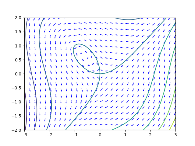
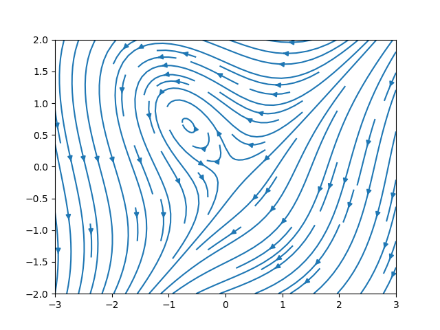
Today we introduced gradient systems which are special planar systems where there is a real valued function such that
Recall from multivariable calulus that the gradient of a function is So in vector form, a gradient system can be expressed as: In a gradient system, the solution curves always try to take the path of steepest ascent up to higher values of .
Calculate the gradient of . Describe the behavior and equilibrium solutions of the gradient system .
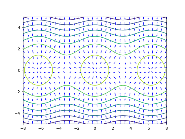
Calculate the gradient of the function .
Sketch some level curves for and then sketch some of the gradient vectors. Use those to describe how different solution curves for the system will behave.
The matrices rotate vectors in to the left and right (respectively) by 90-degrees.
| Day | Section | Topic |
|---|---|---|
| Mon, Nov 17 | 5.2 | Hamiltonian Systems |
| Wed, Nov 19 | Review | |
| Fri, Nov 21 | Midterm 3 | |
| Mon, Nov 23 | 6.1 | The Laplace Transform |
Last time, we ended with a question: what happens if you rotate the direction vectors in a gradient system by 90-degrees to the right? You get a Hamiltonian system. A Hamiltonian system in 2-dimensions is a system of differential equations of the form The function is called the Hamiltonian function for the system. Unlike gradient systems, the solution of a Hamiltonian system move along the level curves of . Therefore the value of is constant on any solution curve. We say that is a conserved quantity for the system.
Show that is a Hamiltonian for the nonlinear pendulum equation We talked about how the terms of the Hamiltonian function for the nonlinear pendulum represent the kinetic energy plus the potential energy of the pendulum.
Consider the system
If this is a Hamiltonian system, then there is a function
such that
and
.
Try to integrate these two formulas to find a function
that works.
The integral of with respect to is where can be any function of . The integral of with respect to is . So a combined solution that works is .
If is the Hamiltonian function of a Hamilton system, then what is the formula for the Jacobian matrix for the system? What can you say about the trace and determinant of the Jacobian matrix?
What types of equilibria are not possible for Hamiltonian systems?
Show that the system is not Hamiltonian by using the fact that in a Hamiltonian system.
Even though this last example is not a Hamiltonian system, it does have a conserved quantity: .
We went over the review problems for midterm 3.
Today we introduced the Laplace transform.
The Laplace transform of a function is
We computed and talked about its domain.
Show that the Laplace transform is linear, i.e.,
After that, we did the following activity about Laplace transforms.
| Day | Section | Topic |
|---|---|---|
| Mon, Dec 1 | 6.1 | The Laplace Transform - con’d |
| Wed, Dec 3 | 6.2 | Solving Initial Value Problems |
| Fri, Dec 5 | 6.2 | Solving Initial Value Problems - con’d |
| Mon, Dec 8 | Recap & review |
When we work with Laplace transforms it is helpful to have a table. Here is a table of common Laplace transforms.
| Original function | Laplace transform | s-Domain |
|---|---|---|
| , | ||
Here are some of the important rules for the Laplace transform.
| Original function | Laplace transform | |
|---|---|---|
| Derivative rules | ||
| Exponential shift rules | ||
After that, we did a quick review of partial fraction decomposition.
Use the partial fraction decomposition to find constants and such that Then use the inverse Laplace transform to solve the differential equation. (https://youtu.be/EdQ7Q9VoF44)
Use the Laplace transform to convert the initial value problem into an algebraic equation, then solve for . (https://youtu.be/qZHseRxAWZ8?t=2203)
Use a computer to find the partial fraction decomposition for .
from sympy import *
s = symbols('s')

# The apart() function in sympy computes the partial fraction decomposition.
print(apart((s**2 + s + 1)/((s+1)**2 * (s-1))))
We finished by talking about the exponential shift rule for Laplace transforms:
Show that .
By definition, .
Use the exponential shift rule to find the inverse Laplace transform of
Today we introduced the Heavyside step function (also known as the unit step function). These are useful because they let us work with differential equations that have discontinuous forcing functions.
Laplace Transform of the Heavyside Function
Second Exponential Shift Formula
Assuming that , find the Laplace transform of this equation.
.
So
.
Find the inverse Laplace transform of . Hint, first find the partial fraction decomposition of
In the partial fraction decomposition, and , so So
After that example, we talked about impulse which is defined as the integral of a force with respect to time. The impulse applied to an object is equal to the object’s change in momentum.
In some situations, we may apply a very large force over a very short
period of time, for example, hitting something with a hammer. In a case
like that, you can model the forcing term using the Dirac delta
function
.
This isn’t really a function itself, but it is a limiting case of the
functions
as
.
The Dirac delta function delivers a total impulse of
instantaneously.
Although
is not technically a function, it still has a nice well-defined Laplace
transform.
The Dirac Delta Function
This is not actually a function, but it has the following properties.
For any continuous function :
Laplace transform.
Intuitively, think of as a function that suddenly delivers an impulse of one at time .
We didn’t get to the next two examples in class today. But they are good practice if you want to try them on your own.
Today we went over Homework 11 before the quiz. Then we talked about the final exam.
Originally, I didn’t put any questions about Euler’s method on the final exam review problems, so we did this example in class.
I’ve actually added that problem to the review problems now and I’ve also posted the solutions.