

| Day | Section | Topic |
|---|---|---|
| Wed, Jan 17 | 1.2 | Floating point arithmetic |
| Fri, Jan 19 | 1.2 | Significant digits, relative error |
We talked about how computers store floating point numbers. Most modern programming languages store floating point numbers using the IEEE 754 standard.
In the IEEE 754 standard, a 64-bit floating point number has the form where
To understand floating point numbers, we also reviewed binary numbers, scientific notation, and logarithmic scales.
We did the following exercises in class:
Convert (10110)2 to decimal. (https://youtu.be/a2FpnU9Mm3E)
Convert 35 to binary. (https://youtu.be/gGiEu7QTi68)
What are the largest and smallest 64-bit floating point numbers that can be stored?
In Python, compute 2.0**1024 and
2**1024. Why do you get different results?
In Python, compare 2.0**1024 with
2.0**(-1024) and 2.0**(-1070). What do you
notice?
Today we talked about significant digits. Here is a quick video on how these work. Then we defined absolute and relative error:
Let be an approximation of .
The base-10 logarithm of the relative error is approximately the number of significant digits, so you can think of significant digits as a measure of relative error. Keep in mind these rules:
Intuitively, addition & subtraction “play nice” with absolute error while multiplication and division “play nice” with relative error. This can lead to problems:
Catastrophic cancellation. When you subtract two numbers of roughly the same size, the relative error can get much worse. For example, both 53.76 and 53.74 have 4 significant digits, but only has 1 significant digit.
Useless precision. If you add two numbers with very different magnitudes, then having a very low relative error in the smaller one will not be useful.
We finished by looking at how you can sometimes re-write algorithms on a computer to avoid overflow/underflow issues. Stirling’s formula is an approximation for which has a relative error that gets smaller as increases.
We used the math library in Python to test
Stirling’s formula, which is the following
approximation
import math
n = 100
print(float(math.factorial(n)))
f = lambda n: math.sqrt(2*math.pi*n)*n**n/math.exp(n)
print(f(n))
Our formula worked well until , then we got an overflow error. The problem was that got too big to convert to a floating point number. But you can prevent the overflow error by adjusting the formula slightly to.
n = 143
f = lambda n: math.sqrt(2*math.pi*n)*(n/math.exp(1))**n
print(f(n))| Day | Section | Topic |
|---|---|---|
| Mon, Jan 22 | Taylor’s theorem | |
| Wed, Jan 24 | Taylor’s theorem - con’d | |
| Fri, Jan 26 | The Babylonian algorithm |
Today we reviewed Taylor series. We recalled the following important Maclaurin series (which are Taylor series with center ):
The we did the following workshop in class.
Today we reviewed some theorems that we will need throughout the course. The first is probably the most important theorem in numerical analysis since it lets us estimate error when using Taylor series approximations.
Taylor’s Theorem. Let be a function that has derivatives in the interval between and . Then there exists a strictly inside the interval from to such that where is the th degree Taylor polynomial for centered at .
A special case of Taylor’s theorem is when . Then you get the Mean Value Theorem (MVT):
Mean Value Theorem. Let be a function that is differentiable in the interval between and . Then there exists a strictly inside the interval from to such that
The proof of both the Mean Value Theorem and Taylor’s Theorem comes from looking at an even simpler theorem called Rolle’s theorem.
Rolle’s Theorem. Let be a function that is differentiable in the interval between and and suppose that . Then there exists a strictly inside the interval from to such that

We briefly sketched an intuitive proof of Rolle’s theorem using the Extreme Value Theorem from calculus, but the details of that proof are not really that important.
We did the following exercises in class.
Use Taylor’s theorem to estimate the error in using the 20th degree Maclaurin series to estimate .
Use Taylor’s theorem to estimate the error in using the 20th degree Maclaurin series to estimate .
We finished with a proof that the number is irrational. First we temporarily assumed that is a reduced fraction . Then we calculated the worst remainder for the th degree Maclaurin polynomial for at . We did the following exercises that lead to a contradiction:
Show that must be an integer.
Use Taylor’s theorem to show that must be strictly between 0 and 1.
Today we did a workshop about the Babylonian algorithm which is an ancient method for finding square roots.
As part of this workshop we also covered how to define variables and functions in Python and also how to use for-loops and while-loops.
| Day | Section | Topic |
|---|---|---|
| Mon, Jan 29 | 2.1 | Bisection method |
| Wed, Jan 31 | 2.3 | Newton’s method |
| Fri, Feb 2 | 2.4 | Rates of convergence |
We talked about how to find the roots of a function. Recall that a root (AKA a zero) of a function is an -value where the function hits the -axis. We introduced an algorithm called the Bisection method for finding roots of a continuous function. We did the following workshop.
One feature of the Bisection method is that we can easily find the worst case absolute error in our approximation of a root. That is because every time we repeat the algorithm and cut the interval in half, the error reduces by a factor of 2, so that We saw that it takes about 10 iterations to increase the accuracy by 3 decimal places (because ).
We finished by comparing the bisection method for finding roots with the Babylonian algorithm for finding square roots. Why are square roots called roots? Because every square root is a root of a square function. For example, is a root of .
Today we covered Newton’s method. This is probably the most important method for finding roots of differentiable functions. The formula is This formula comes from the idea which is to start with a guess for a root and then repeatedly improve your guess by following the tangent line at until it hits the -axis.
Use Newton’s method to find roots of .
How can you use Newton’s method to find ? Hint: use .
Theorem. Let and suppose that has a root . Suppose that there are constants such that and for all . Then when .
Proof. Start with the first degree Taylor polynomial (centered at ) for including the remainder term and the Newton’s method iteration formula:
and
Subtract these two formulas to get a formula that relates with .
Use this to get an upper bound on . □
Corollary. The error in the -th iterate of Newton’s method satisfies
This corollary explains why, if you start with a good guess in Newton’s method, the number of correct decimal places tends to double with each iteration!
Today we looked at some examples of what can go wrong with Newton’s method. We did these examples:
What happens if you use Newton’s method with on ?
Why doesn’t Newton’s method work for ?
We also did this workshop.
| Day | Section | Topic |
|---|---|---|
| Mon, Feb 5 | 2.5 | Secant method |
| Wed, Feb 7 | 2.2 | Fixed point iteration |
| Fri, Feb 9 | 2.4 | More about rates of convergence |
We talked about the secant method which is a variation of Newton’s method that uses secant lines instead of tangent lines. The advantage of the secant method is that it doesn’t require calculating a derivative. The disadvantage is that it is a little slower to converge than Newton’s method, but it is still much faster than the bisection method. Here is the formula:
We wrote the following program in class.
def Secant(f, a, b, precision = 10**(-8)):
    while abs(b-a) > precision:
        a, b = b, b - f(b)*(b-a)/(f(b)-f(a))
    return b
Sometimes a function might be very time consuming for a computer to compute, so you could improve this function by reducing the number of times you have to call . If speed is a concern, then this would be a better version of the function.
def Secant(f, a, b, precision = 10**(-8)):
    fa = f(a)
    fb = f(b)
    while abs(b-a) > precision:
        a, b = b, b - fb*(b-a)/(fb-fa) # update x-values
        fa, fb = fb, f(b) # update y-values using the new x-value
    return b
Notice how we call the function
three times in each iteration of the while-loop in the first program,
but by storing the result in the variables fa and
fb, we only have to call
once per iteration in the second version of the program.
We finished by talking about the convergence rate of the secant method.
Theorem. Let and suppose that has a root . There is a constant such that for , sufficiently close to (say and ), the next iterate of the secant method has In particular, will converge to .
Note, the constant might be larger than the constant from Newton’s method, but it is usually not much larger.
We saw that the pattern is that the exponents of each factor is a Fibonacci number. We talked briefly about Binet’s formula for Fibonacci numbers and the golden ratio . The lead to the following nice rule of thumb: The number of correct decimal places in the secant method increases by a factor of about 1.6 (the golden ratio) every step.
Newton’s method is a special case of a method known as fixed point iteration. A of a function is a number such that . Not every function has a fixed point, but we do have the following existence result:
Theorem. Let . If for every , then must have a fixed point in .
Show that has a fixed point in .
Explain why has no fixed points.
A fixed point is attracting if for all sufficiently close to , the recursive sequence defined by converges to . It is repelling if no (sub)sequence of ever converges to . You can draw a picture of these fixed point iterates by drawing a cobweb diagram.

Show that the fixed point of is attracting by repeatedly iterating.
Show that has a fixed point, but it is not attracting.
Theorem If has a fixed point and
You can sometimes use fixed point iteration to solve equations. For example, here are two different ways to solve the equation using fixed point iteration.
Re-write the equation as .
Replace with the equation where is a small constant. The constant works well for the function above.
When a sequence converges to a root , we say that it has a linear order of convergence if there is a constant such that We say that the sequence has a quadratic order of convergence if there is a constant such that More generally, a sequence converges with order if there is are constants and such that
In general, a sequence that converges with order will have the number of correct decimal places grow by a factor of about each step. Newton’s method is order 2, Secant method is order , and the Bisection method is only linear order.
Theorem. If is differentiable at a fixed point and , then for any point sufficiently close to , the fixed point iterates defined by converge to with linear order. If , then the iterates converge to with order where is the first nonzero derivative of at .
We started with this question:
Then we did this workshop in class.
In one step of the workshop, we used the triangle inequality which says that for any two numbers and ,
| Day | Section | Topic |
|---|---|---|
| Mon, Feb 12 | Systems of linear equations | |
| Wed, Feb 14 | LU decomposition | |
| Fri, Feb 16 | Matrix norms |
Today we talked about systems of linear equations and linear algebra. Before we got to that, we looked at one more cool thing about Newton’s method. It also works for to find complex number roots if you use complex numbers. We talked about the polynomial which has three roots: and . We talked about which complex numbers end up converging to which root as you iterate Newton’s method. You get a beautiful fractal pattern:

After that we started a review of row reduction from linear algebra.
We can represent this question as a system of linear equations. where are the numbers of pennies, nickles, dimes, and quarters respectively. It is convenient to use matrices to simplify these equations: Here we have a matrix equation of the form where , is the unknown vector, and . Then you can solve the problem by row-reducing the augmented matrix
which can be put into echelon form
Then the variables , and are pivot variables, and the last variable is a free variable. Each pivot variable depends on the value(s) of the free variables. A solution of a system of equations is a formula for the pivot variables as functions of the free variables.
Recall the following terminology from linear algebra. For any matrix (i.e., that has real number entries with rows and columns):
The rank of is the number of pivots. It is also the dimension of the column space since the columns of with pivots are linearly independent and form a basis for the column space.
The null space of is the set .
The nullity of is the number of free variables which is the same as the dimension of the null space of .
Rank + Nullity Theorem. Let . Then the rank of plus the nullity of must equal .
A matrix equation has a solution if and only if is in the column space of . If is in the column space, then there will be either one unique solution if there are no free variables (i.e., the nullity of is zero) or there will be infinitely many solutions if there are free variables.
If
(i.e.,
is a square matrix) and the rank of
is
,
then
is invertible which means that there is a matrix
such that
where
is the identity matrix
You can use row-reduction to find the inverse of an invertible matrix by
row reducing the augmented matrix
until you get
.
Use row-reduction to find the inverse of . (https://youtu.be/cJg2AuSFdjw)
Use the inverse to solve .
In practice, inverse matrices are rarely used to solve systems of linear equations for a couple of reasons.
Today we talked about LU decomposition. We defined the LU decomposition as follows. The LU decomposition of a matrix is a pair of matrices and such that and is in echelon form and is a lower triangular matrix with 1’s on the main diagonal, 0’s above the main diagonal, and entries in row , column that are equal to the multiple of row that you subtracted from row as you row reduced to .
Compute the LU decomposition of .
Use the LU decomposition to solve .
We also did this workshop.
We finished with one more example.
Today we talked about what it means for a linear system to be ill-conditioned. This is when a small change in the vector can produce a large change in the solution vector for a linear system .
Consider the following matrix:
Let and .
Consider the matrix
which has
decomposition
Although
is not ill-conditioned, you have to be careful using row reduction to
solve equations with this matrix because both
and
in the LU-decomposition for
are ill-conditioned.
A norm is a function from a vector space to with the following properties:
Intuitively a norm measures the length of a vector. But there are different norms and they measure length in different ways. The three most important norms on the vector space are:
The -norm (also known as the Euclidean norm) is the most commonly used, and it is exactly the formula for the length of a vector using the Pythagorean theorem.
The -norm (also known as the Manhattan norm) is This is the distance you would get if you had to navigate a city where the streets are arranged in a rectangular grid and you can’t take diagonal paths.
The -norm (also known as the Maximum norm) is
These are all special cases of -norms which have the form
We used Desmos to graph the set of vectors in with -norm equal to one, then we could see how those norms change as varies between 1 and .
The set of all matrices in
is a vector space. So it makes sense to talk about the norm of a matrix.
There are many ways to define norms for matrices, but the most important
for us are operator norms (also known as
induced norms). For a matrix
,
the induced
-norm
is
Two important special cases are
For an invertible matrix , the condition number of is (using any induced norm).
Rule of thumb. If the entries of and are both accurate to -significant digits and the condition number of is , then the solution of the linear system will be accurate to significant digits.
| Day | Section | Topic |
|---|---|---|
| Mon, Feb 19 | Condition numbers | |
| Wed, Feb 21 | Review | |
| Fri, Feb 23 | Midterm 1 |
Theorem. If is invertible, then the relative error in the solution of the system is bounded by
Proof. Using the properties of the induced norm,
so putting both together gives
This leads directly to the inequality above when you separate the
factors with
from those with
.
□
This explains why the number of significant digits in the solution to may have up to fewer significant digits than the entries of and when the condition number .
Last time we saw an example of a matrix which is not ill-conditioned by itself. However, both and in its LU-decomposition were ill-conditioned. It is possible to avoid this problem using the method of partial pivoting. The idea is simple: when more than one entry could be the pivot for a column, always choose the one with the largest absolute value.
You keep track of the row swaps as you use the method of partial pivoting, always apply the same row swaps to a copy of the identity matrix. At the end, you will have a permutation matrix and the LU-decomposition with partial pivoting is The fixes two problems:
One nice thing to know about permutation matrices is that they are always invertible and where is the transpose of obtained by converting every row of to a column of .
Find the LU-decomposition with partial pivoting for these matrices
Today we reviewed for the midterm exam. We reviewed the things you need to memorize. We also talked about the following problems.
Find the LU decomposition of .
Find and classify the fixed points of . This was a little hard to solve, because it isn’t easy to factor the polynomial . But it does have computable roots and .
How would you use secant method to find the one negative root of ? What would make good choices for and ? What is for those choices?
If and , then how many significant digits do the following have?
| Day | Section | Topic |
|---|---|---|
| Mon, Feb 26 | 3.1 | Polynomial interpolation, Vandermonde matrices |
| Wed, Feb 28 | 3.1 | Polynomial bases, Lagrange & Newton polynomials |
| Fri, Mar 1 | 3.2 | Newton’s divided differences |
Today we started talking about polynomial interpolation. An interpolating polynomial is a polynomial that passes through a set of points in the coordinate plane. We started with an example using these four points: , , , and .
In order to find the interpolating polynomial, we introduced Vandermonde matrices. For any set of fixed -values, , the Vandermonde matrix for those values is the matrix such that the entry in row and column is In other words, looks like Notice that when working with Vandermonde matrices, we always start counting the rows and columns with .
Using the Vandermonde matrix , we can find an -th degree polynomial that passes through the points by solving the system where is the vector of coefficients and is the vector with -values corresponding to each . That is, we want to solve the following system of linear equations:
In Python with the Numpy library, you can enter a Vandermonde matrix using a list comprehension inside another list comprehension. For example, the Vandermonde matrix for -values can be entered as follows.
import numpy as np
V = np.array([[x**k for k in range(4)] for x in [-1,0,1,5]])
Then the function np.linalg.solve(V,y) will solve the
system
.
For example, after entering
,
we would solve the first example as follows.
y = np.array([-4, 3, 0 8])
a = np.linalg.solve(V,y)
print(a) # prints [ 3.  1. -5.  1.]
Therefore the solution is
After that example, we did the following examples in class.
Find an interpolating polynomial for these points: , , , and
Find a 4th degree polynomial that passes through , , , ,
Last time, when we talked about polynomial interpolation, we wrote our interpolating polynomials as linear combinations of the standard monomial basis for the space of all -th degree polynomials. There are other bases we could choose. Today we introduce two alternative bases: the Lagrange polynomials and the Newton polynomials. Both require a set of distinct -values called nodes, . For any given set of nodes, the Lagrange polynomials are The defining feature of the Lagrange polynomials is that From this we saw that the interpolating polynomial passing through is
Find the Lagrange polynomials for the nodes .
Use those Lagrange polynomials to find the interpolating polynomial that passes through .
Express the interpolating polynomial that passes through as a linear combination of Lagrange polynomials.
We finished by describing the Newton polynomials which are
You can express an interpolating polynomial as a linear combination of Newton polynomials by solving the linear system
to find coefficients such that the interpolating polynomial passes through each point .
Today we talked about the method of divided differences, which lets us find the coefficients of an interpolating polynomial expressed using the Newton basis.
For a function and a set of distinct -values, , the divided differences are defined recursively by the following formula
We did these examples.
Make a divided differences table for the points , and use it to find the interpolating polynomial (in Newton form).
Use the -values , , , , to make an interpolating polynomial for
Solution
The table of divided differences is:
|
DD1 |
DD2 |
DD3 |
DD4 |
||
So the Newton form of the interpolating polynomial is Notice that the coefficients are just the numbers (in blue) at the top of each column in the divided differences table.
Here are some videos with additional examples:
After those examples, we did this workshop in class:
| Day | Section | Topic |
|---|---|---|
| Mon, Mar 4 | 3.3 | Interpolation error |
| Wed, Mar 6 | 3.3 | Interpolation error - con’d |
| Fri, Mar 8 | 3.4 | Chebyshev polynomials |
Often the interpolating polynomial is constructed for a function so that for each node . Then we call an interpolating polynomial for the function . Using interpolating polynomials is one way to approximate a function. For example, we did this last time with the function .
Here are some important results about these approximations.
Mean Value Theorem for Divided Differences. Let be distinct nodes in and let . Then there exists a number between the values of such that
Proof. Let be the -th degree interpolating polyomial for at . The function has roots, so its derivative must have roots, and so on, until the n-th derivative has at least one root. Call that root . Then . However, is a linear combination of Newton basis polynomials and only the last Newton basis polynomial is -th degree. Its coefficient in the interpolating polynomial is so when you take derivatives of , you get which completes the proof. □
Interpolation Error Theorem. Let be distinct nodes in and let . If is the -th degree interpolating polynomial for those nodes, then for each , there exists a number between , and such that
Proof. Add to the list of nodes and construct the -th degree interpolating polynomial . Then using the Newton form for both interpolating polynomials, So by the MVT for Divided Differences, there exists between and such that
We finished with the following example.
Today we looked at some interpolation examples in more detail. We used Python to implement the Vandermonde matrix and the divided difference methods for finding interpolating polynomials. Then we use the following Python notebook to look at some of the issues that arise with interpolation.
In the notebook, we looked at the following two examples which both raise important issues.
on . This example illustrates what goes wrong when you use the Vandermonde matrix approach. As the number of nodes grows past 20, the Vandermonde matrix is ill-conditioned, so it gives an incorrect interpolating polynomial. Because large Vandermonde matrices tend to be ill-conditioned, using the method of divided differences with the Newton basis for interpolation is usually preferred.
on . This function is a version of Runge’s function (also known as the Witch of Agnesi).
When you use equally spaced nodes interpolate the function on , the error gets worse as the number of nodes increases, particularly near the endpoints of the interval. This problem is called Runge’s phenomenon.
It is possible to avoid the error from Runge’s phenomenon. The key is to use a carefully chosen set of nodes that are not equally spaced. The best nodes to use are the roots of the Chebyshev polynomials which (surprisingly!) are equal to the following trigonometric functions on the interval : The roots of the th degree Chebyshev polynomials are:
Today we wrapped up our discussion of polynomial interpolation with this workshop.
| Day | Section | Topic |
|---|---|---|
| Mon, Mar 18 | 5.1 | Newton-Cotes formulas |
| Wed, Mar 20 | 5.1 | Newton-Cotes formulas - con’d |
| Fri, Mar 22 | Error in Newton-Cotes formulas |
Today we introduced numerical integration. We reviewed the Riemann sum definition of the definite integral where is the number of rectangles, , and is the right endpoint of each rectangle. Then we talked about the following methods for approximating integrals:
We derived the formulas for the composite trapezoid rule
and the composite Simpson’s rule
where and in both formulas. Here is an example of a Python function that computes the composite Simpson’s rule:
def simpson(f, a, b, n):
  h = (b-a)/n
  total = f(a)+f(b)
  total += sum([4*f(a+(k+0.5)*h) for k in range(n)])
  total += sum([2*f(a+k*h) for k in range(1,n)])
  return total*h/6
We looked at this example in class:
Today we did the following workshop about numerical integration.
Here are some tips for the workshop.
You might want to review the Taylor series workshop we did all the way back on January 22.
Because the function is undefined at , you will get an error if you ask Python to evaluate the function there (for example, in problem 4). To avoid that problem, you can use this code to define :
from math import *

f = lambda x: sin(x)/x if x != 0 else 1Today we talked about the error in Newton-Cotes integration methods. An integration method has degree of precision if it is perfectly accurate for all polynomials up to degree . It is easy to see that the trapezoid method has degree of precision 1. Surprisingly, Simpson’s method has degree of precision 3.
Theorem. Simpson’s method has degree of precision 3.
We proved this theorem in class by observing that if
is a third degree polynomial and
is a second degree interpolating polynomial for
at the nodes
,
,
and
then
where
is the third divided difference
.
Then we used u-substitution to show that
Since Simpson’s method is just the integral of
and the extra term integrates to zero, it follows that Simpson’s method
is exact for 3rd degree polynomials.
For most other functions, Simpson’s method will not be perfect. Instead, we can use the error formulas for polynomial interpolation to estimate the error when using the composite trapezoid and Simpson’s methods. Here are the error formulas:
Composite Trapezoid Rule Error.
Composite Simpson’s Rule Error.
We didn’t prove the Simpson’s rule error formula in class, but we did prove the error formula for the trapezoid rule and the proof for Simpson’s rule is similar. We finished by applying these rules to the following questions:
How big does need to be in the composite trapezoid rule to estimate with an error of less than ?
How big does need to be in the composite trapezoid rule to estimate with an error of less than ?
If you double , how much does the error tend to decrease in the trapezoid rule? What about in the Simpon’s rule?
| Day | Section | Topic |
|---|---|---|
| Mon, Mar 25 | 5.4 | Gaussian quadrature |
| Wed, Mar 27 | 5.6 | Monte carlo integration |
| Fri, Mar 29 | 4.1 | Numerical differentiation |
Today we introduced a different numerical integration technique called Gaussian quadrature. This technique is a little more complicated than Simpson’s method, but it can potentially be much more accurate and faster to compute. The idea is that instead of using equally spaced nodes like in the composite Newton-Cotes formulas, you can use a specially chosen set of nodes that allows you to get a degree of precision of with only nodes.
The simplest version of Gaussian quadrature only works on the interval . To apply it to any other interval, you would have to use a change of variables. The formula for Gaussian quadrature is
where are the roots of the nth-degree Legendre polynomial and are special weights that are usually pre-computed.
Here is a table with the values of and for up to 5 from Wikipedia:
| Nodes | Weights | |||
|---|---|---|---|---|
| 1 | 0 | 2 | ||
| 2 | ±0.57735… | 1 | ||
| 3 | 0 | 0.888889… | ||
| ±0.774597… | 0.555556… | |||
| 4 | ±0.339981… | 0.652145… | ||
| ±0.861136… | 0.347855… | |||
| 5 | 0 | 0.568889… | ||
| ±0.538469… | 0.478629… | |||
| ±0.90618… | 0.236927… | |||
We did the following exercises in class.
Use Gaussian quadrature with to estimate .
Use Gaussian quadrature with to estimate
Use the u-substitution to convert the integral into one where you can apply Gaussian quadrature.
What u-substitution could you apply to so that you could apply Gaussian quadrature?
Show that if where and , then
Today we talked about Monte Carlo integration, which is when you randomly generate inputs to try to find the value of an integral. Monte Carlo integration is slow to converge and it can give very bad results if you use a poorly chosen pseudo-random number generator. But it is one of the most effective methods for calculating multivariable integrals.
For a function
,
the basic idea is to calculate the average value of a function in a
region
by randomly generating points
in
.
If the dimension
,
then the double integral over the region
is approximately
and if
,
then the triple integral over
would be
Integrals in higher dimensions are similar, just using higher
dimensional analogues of volume (called the measure of
).
We did this example:
Use Monte Carlo integration to estimate the double integral
Use Monte Carlo integration to estimate the double integral where .
The method above assumes that we choose our points uniformly in . But we can actually use any probability distribution with support equal to to approximate an integral. This is called importance sampling. If we have a method to compute random vectors in with a probability distribution that has density function , then the importance sample formula is: If we randomly generate the coordinates of using a probability distribution like the normal distribution that has unbounded support, then we can calculate improper integrals like this example:
The actual value of this integral should be . In theory, Monte Carlo integration will give the correct answer on average. But in practice using the normal distribution doesn’t work well for this integral because it under-samples the tails. A better probability distribution would be something like the Cauchy distribution or the Pareto distribution which we used in class. It can be tricky to pick a good distribution to use.
Today we talked about numerical differentiation and why it is numerically unstable which means that we can’t use a single numerical technique to get better and better approximations.
Recall that computers represent floating point numbers in binary in the following form: When a computer computes a function, it will almost always have to round the result since there is no where to put the information after the last binary decimal point. So it will have a relative error of about . This number is called the machine epsilon (and denoted ). It is the reason that numerical differentiation techniques are numerically unstable.
When you compute the difference quotient to approximate , the error should be for some between and by the Taylor remainder theorem. But that error formula assumes that and are being calculated precisely. In fact, they are going to have rounding errors and so will only be accurate to approximately where is machine epsilon. Adding that factor, you get a combined error of roughly That explains why the error initially decreases, but then starts to increase as get’s smaller. We graphed the logarithm of the relative error in using the difference quotient to approximate the derivative of as a function of when . To graph it, we introduced the pyplot library in Python:
import matplotlib.pyplot as plt
from math import *

f = lambda x: 10**x
rel_error = lambda h: abs((f(0+h)-f(0))/h - log(10))/log(10)

xs = [k/10 for k in range(180)]
ys = [log(rel_error(10**(-x)))/log(10) for x in xs]

plt.plot(xs,log_rel_errors)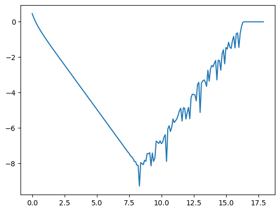
We finished by getting started on this workshop:
| Day | Section | Topic |
|---|---|---|
| Mon, Apr 1 | class canceled | |
| Wed, Apr 3 | Discrete least squares regression | |
| Fri, Apr 5 | Discrete least squares - con’d |
Today we introduced least squares regression. We
took a linear algebra approach to understanding least squares
regression. Given an
-by-
matrix
and a vector
,
we can try to find solutions to the system of equations
But a solution only exists if
is in the column space of
(also known as the range of
).
If
is not in the column space, then there is no solution, but you can
always find a point
such that
is as close as possible to
.
In other words, you can find
that minimizes
where the norm is the
-norm:
That’s why we say we are finding the smallest sum of squared
error.
It is a geometry fact that
is minimized exactly when
is orthogonal to the column space of
.
And that happens exactly when
This is because of the fundamental theorem of linear algebra:
The Fundamental Theorem of Linear Algebra. Let be any -by- matrix. Then
Substituting and rearranging terms, we get the normal equations. You can solve the normal equations using row reduction to find the coefficients of the vector that generate the closest to .
We applied this technique to the examples in this workshop.
Today we talked some more about least squares regression. We started with this warm-up problem.
Then we defined the orthogonal complement of a subspace to be the set of vectors in that are orthogonal to every element in , i.e.,
Use Desmos-3d to graph and for the matrix above.
Find the least squares solution to .
Then we talked about how you can use least squares regression to find the best coefficients for any model, even nonlinear models, as long as the model is a linear function of the coefficients. For example, if you wanted to model daily high temperatures in Farmville, VA as a function of the day of the year (from 1 to 365), you could use a function like this:
Here is the code we used to analyze this example.
import numpy as np
import pandas as pd
import matplotlib.pyplot as plt
from math import *
df = pd.read_excel("http://people.hsc.edu/faculty-staff/blins/StatsExamples/FarmvilleHighTemps2019.xlsx")
xs = np.array(df.day)
ys = np.array(df.high)
plt.plot(xs,ys,"o")
plt.show()

X = np.array([[1, x, cos(2*pi*x/365), sin(2*pi*x/365) ] for x in xs])
bs = np.linalg.solve(X.T @ X, X.T @ ys)
print(bs)

model = lambda t: bs[0]+bs[1]*t + bs[2]*cos(2*pi*t/365) + bs[3]*sin(2*pi*t/365)
plt.plot(xs,ys,"o")
plt.plot(xs, [model(x) for x in xs])
plt.show()
We didn’t have time to do an example of this in class, but here is another nice idea. For models that aren’t linear functions of the parameters, you can often change them into a linear model by applying a log-transform. For example, an exponential model can be turned into a linear model after we take the (natural) logarithm of both sides:
| Day | Section | Topic |
|---|---|---|
| Mon, Apr 8 | Continuous least squares | |
| Wed, Apr 10 | Orthogonal functions, Gram-Schmidt | |
| Fri, Apr 12 | Fourier series |
Today we introduced the idea of continuous least squares regression. Unlike the discrete case where we only want the smallest sum of squared residuals at a finite number of points, here the goal is to find a polynomial that minimizes the integral of the squared differences:
Before we derived the normal equations for continuous least squares regression, we started with a brief introduction to functional analysis (which is like linear algebra when the vectors are functions).
Definition. An inner-product space is a vector space with an inner-product which is a real-valued function such that for all and
The norm of a vector in an inner-product space is .
Examples of inner-product spaces include
Definition. Let be inner-product spaces. If is a linear transformation, then the adjoint of is a linear transformation defined by for every and .
Definition. Let be an inner-product space. Two vectors are orthogonal if . If is a subspace of , then orthogonal complement is the subspace containing all vectors in that are orthogonal to every element of . That is,
The following theorem says that the orthogonal complement of the range of a linear transformation is always the null space of the adjoint.
Theorem. Let be inner-product spaces. If is a linear transformation, then
We want to find the best fit polynomial of degree n.
This polynomial will be in
and it is a linear function of the coefficients
.
So there is a linear transformation
such that
.
We want to find the
closest to
in
.
In other words, we want to minimize
That happens when
is orthogonal to the range of
which happens when
By replacing
with
,
we get the normal equation for continuous least squares
regression:
Since and , the composition is a linear transformation from to . So it is an -by- matrix and its -entry is where are the standard basis vectors for . The entries of are
To summarize, the normal equation to find the coefficients of the continuous least squares polynomial is
Theorem (Continuous Least Squares). For , the coefficients of the continuous least squares polynomial approximation can be found by solving the normal equation where is an -by- matrix with entries and is a vector in with entries
We used this Python code to solve the problem and graph the solution:
import numpy as np
from scipy.integrate import quad
import matplotlib.pyplot as plt

n=2
f = np.exp
left, right = 0, 2
XstarX = np.array([[quad(lambda x: x**(i+j),left,right)[0] for j in range(n+1)] for i in range(n+1)])
Xstarf = np.array([quad(lambda x: x**i*f(x),left,right)[0] for i in range(n+1)])

b = np.linalg.solve(XstarX,Xstarf)
p = lambda x: sum([b[i]*x**i for i in range(n+1)])
print(b)

xvals = np.linspace(left,right,1000) #generates 1000 equally spaced points b/w left & right
plt.plot(xvals,f(xvals))
plt.plot(xvals,p(xvals))
plt.show()Last time we derived the normal equations for continuous least squares. We came up with the following result using the standard basis , but it would work for any linearly independent family of functions in .
Theorem (Continuous Least Squares). For , the coefficients of the continuous least squares polynomial approximation can be found by solving the normal equation where is an -by- matrix with entries and is a vector in with entries
The functions can be any basis of polynomials (i.e., the standard basis, the Lagrange basis, the Newton basis, etc.) But the nicest basis for this formula would be if the polynomials were all orthogonal to each other. In linear algebra there is an algorithm to take a set of vectors that aren’t all orthogonal, and create a new set of vectors with the same span that are all orthogonal to each other.
Gram-Schmidt Algorithm. Given a set of linearly independent vectors in an inner product space , this will find a set of pairwise orthogonal vectors that have the same span as the original vectors.
Let .
For each , let
If we have an orthogonal basis of functions , such as the Legendre polynomials, then the matrix from the normal equation has zero entries except on the main diagonal:
Therefore the solution of the normal equations is just
We used Desmos to compute the 2nd degree continuous least squares regression polynomial on the interval using the Legendre basis polynomials for the following functions.
.
.
Today we talked about Fourier series. The Legendre polynomials on the interval aren’t the only example of an orthogonal set of functions. Probably the most important example of an orthogonal set of functions is the set on the interval . Any function in can be approximated by using continuous least squares with these trig functions. Since there are an infinite number of functions in this orthogonal set, we usually stop the approximation when we reach a high enough frequency and .
We started by using the trig product formulas to find the norms of and for any . We also proved that is orthogonal to when .
Then we did this workshop.
| Day | Section | Topic |
|---|---|---|
| Mon, Apr 15 | Review | |
| Wed, Apr 17 | Midterm 2 | |
| Fri, Apr 19 | 6.1 | Euler’s method |
Today we reviewed for midterm 2. Instead of going over the review problems, we talked about the formulas you should have memorized (most other formulas will be given with the problem, although you will have to know how to use them). Here was the list we came up with:
Vandermonde matrices & the standard basis for polynomials
Lagrange basis
Divided differences and the Newton basis
The difference quotient
Inner-product and norm for .
Degree of precision for integration methods
We did the following exercises.
Use divided differences to find the interpolating polynomial for the points and .
Use the Langrange basis to find the same interpolating polynomial.
What Vandermonde matrix would you use, and in what linear system, to find the coefficients of the interpolating polynomial in the standard basis.
What would you get if you used Gaussian quadrature with nodes to calculate ?
We also mentioned a few other important concepts that you might want to review like:
Runge’s phenomenon - Where interpolating polynomials don’t always get more accurate as you use more an more nodes.
Machine epsilon ( for double precision floats which are standard in most programming languages including Python and Javascript) - This is the most accurate the computer can be when it rounds calculations using floating point numbers.
Numerical instability - Some formulas (like the formulas for approximating derivatives) do not get more accurate as you increase the precision past a certain threshold.
We talked more about the Initial Value Problem (abbreviated IVP) for first order differential equations (abbreviated ODEs).
We started with this example:
Then we introduced the following theorem (without proof):
Theorem (Existence & Uniqueness of Solutions). If is continuous and the partial derivatives are bounded for all , then the initial value problem has a unique solution defined on the interval .
We looked at these examples:
The differential equation has solutions that follow circular arcs centered at the origin. The IVP has two solutions and . Why doesn’t that contradict the theorem above? Which condition of the theorem fails for this IVP?
The explosion equation is the ODE The solution is . If , then a solution to the IVP with is . But that solution is not defined when (it has a vertical asymptote). Why is that consistent with the theorem above?
Show that is the unique solution of the IVP with . How do you know that this is the only solution?
Unfortunately most differential equations cannot be solved analytically (the way we did for the examples above). So next week, we will talk about methods to find approximate solutions.
| Day | Section | Topic |
|---|---|---|
| Mon, Apr 22 | 6.1 | Euler’s method error |
| Wed, Apr 24 | Existence & uniqueness of solutions | |
| Fri, Apr 26 | 6.4 | Runge-Kutta methods |
| Mon, Apr 29 | Review |
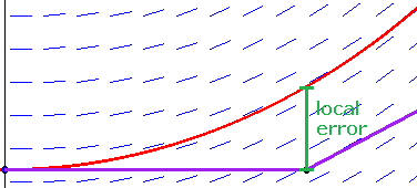
The simplest method for finding an approximate solution to a differential equation is Euler’s method.
To find an approximate solution to the initial value problem on the interval ,
We started by doing this example by hand:
Then we implemented the algorithm in Python to get a more accurate solution.
from math import *
import matplotlib.pyplot as plt

def EulersMethod(f,a,b,h,y0):
    # Returns two lists, one of t-values and the other of y-values.
    t, y = a, y0
    ts, ys = [a], [y0]
    while t < b:
      y += f(t,y)*h
      t += h
      ts.append(t)
      ys.append(y)
    return ts, ys

f = lambda t,y: y-t**2 + 1

# h = 1
ts, ys = EulersMethod(f,-1,3,1,0)
plt.plot(ts,ys)
# h = 0.1
ts, ys = EulersMethod(f,-1,3,0.1,0)
plt.plot(ts,ys)
# h = 0.01
ts, ys = EulersMethod(f,-1,3,0.01,0)
plt.plot(ts,ys)
plt.show()To analyze the population example we used this Python code:
f = lambda t,y: 0.1*y*(10+2*cos(2*pi*t)-y)
# h = 1
ts, ys = EulersMethod(f,0,10,1,1)
plt.plot(ts,ys)
# h = 0.1
ts, ys = EulersMethod(f,0,10,0.1,1)
plt.plot(ts,ys)
# h = 0.01
ts, ys = EulersMethod(f,0,10,0.001,1)
plt.plot(ts,ys)
plt.show()We started with this question:
Over many steps, the error from using Euler’s method tends to grow. It is possible to prove the following upper bound for the error in Euler’s method over the whole interval :
where , , and is machine epsilon. At first, the error decreases as gets smaller, but eventually the machine epsilon term (which comes from rounding errors) gets very large, so Euler’s method can be numerically unstable.
To get a method with less error, would could try to incorporate the 2nd derivative of into each step. Note that by the chain rule for multivariable functions. In practice it isn’t always easy to compute the partial derivatives of , so the Runge-Kutta method looks for relatively simple formulas involving that approximate this expression above without calculating the partial derivatives. The 2nd order Runge-Kutta method known as the midpoint method has this formula
Second Order Runge-Kutta Algorithm. To approximate a solution to the IVP on the interval ,
We implemented the algorithm for this Runge-Kutta method in Python and used it to approximate the solution of this IVP:
We also compared our result with the Euler’s method approximate solutions for and . We saw that the midpoint method was much more accurate. My version of the code for this algorithm is below.
def MidpointMethod(f,a,b,h,y0):
    # Return two lists, one of y-values and the other of t-values
    t, y = a, y0
    ts, ys = [a], [y0]
    while t < b:
      y += f(t+h/2,y+h/2*f(t,y))*h
      t += h
      ts.append(t)
      ys.append(y)
return ts, ysToday we introduced the 4th order Runge-Kutta (RK4) method and we did this workshop:


